Download
1 / 50
500 likes | 679 Views
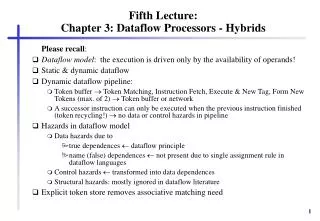
Fifth Lecture: Chapter 3: Dataflow Processors - Hybrids. Please recall : Dataflow model : the execution is driven only by the availability of operands! Static & dynamic dataflow Dynamic dataflow pipeline:

E N D
Fifth Lecture:Chapter 3: Dataflow Processors - Hybrids Please recall: • Dataflow model: the execution is driven only by the availability of operands! • Static & dynamic dataflow • Dynamic dataflow pipeline: • Token buffer Token Matching, Instruction Fetch, Execute & New Tag, Form New Tokens (max. of 2) Token buffer or network • A successor instruction can only be executed when the previous instruction finished (token recycling!) no data or control hazards in pipeline • Hazards in dataflow model • Data hazards due to • true dependences dataflow principle • name (false) dependences not present due to single assignment rule in dataflow languages • Control hazards transformed into data dependences • Structural hazards: mostly ignored in dataflow literature • Explicit token store removes associative matching need
Augmenting Dataflow with Control-Flow • poor sequential code performance by dynamic dataflow computers • Why? • an instruction of the same thread is issued to the dataflow pipeline after the completion of its predecessor instruction. • In the case of an 8-stage pipeline, instructions of the same thread can be issued at most every eight cycles. • Low workload: the utilization of the dataflow processor drops to one eighth of its maximum performance. • Another drawback: the overhead associated with token matching. • before a dyadic instruction is issued to the execution stage, two result tokens have to be present. • The first token is stored in the waiting-matching store, thereby introducing a bubble in the execution stage(s) of the dataflow processor pipeline. • measured pipeline bubbles on Monsoon: up to 28.75 % • no use of registers possible!
Augmenting Dataflow with Control-Flow • Solution: combine dataflow with control-flow mechanisms: • threaded dataflow, • large-grain dataflow, • dataflow with complex machine operations, • further hybrids
Threaded Dataflow • Threaded dataflow: the dataflow principle is modified so that instructions of certain instruction streams are processed in succeeding machine cycles. • A subgraph that exhibits a low degree of parallelism is transformed into a sequential thread. • The thread of instructions is issued consecutively by the matching unit without matching further tokens except for the first instruction of the thread. • Threaded dataflow covers • the repeat-on-input technique used in Epsilon-1 and Epsilon-2 processors, • the strongly connected arc model of EM-4, and • the direct recycling of tokens in Monsoon.
Threaded Dataflow (continued) • Data passed between instructions of the same thread is stored in registers instead of written back to memory. • Registers may be referenced by any succeeding instruction in the thread. • Single-thread performance is improved. • The total number of tokens needed to schedule program instructions is reduced which in turn saves hardware resources. • Pipeline bubbles are avoided for dyadic instructions within a thread. • Two threaded dataflow execution techniques can be distinguished: • direct token recycling (Monsoon), • consecutive execution of the instructions of a single thread (Epsilon & EM).
Direct token recycling of Monsoon • Cycle-by-cycle instruction interleaving of threads similar to multithreaded von Neumann computers! • 8 register sets can be used by 8 different threads. • Dyadic instructions within a thread (except for the start instruction!) refer to at least one register, need only a single token to be enabled. • A result token of a particular thread is recycled ASAP in the 8-stage pipeline, i.e. every 8th cycle the next instruction of a thread is fired and executed. • This implies that at least 8 threads must be active for a full pipeline utilization. • Threads and fine-grain dataflow instructions can be mixed in the pipeline.
Epsilon and EM-4 • Instructions of a thread are executed consecutively. • The circular pipeline of fine-grain dataflow is retained. • The matching unit is enhanced with a mechanism that, after firing the first instruction of a thread, delays matching of further tokens in favor of consecutive issuing of all instructions of the started thread. • Problem: implementation of an efficient synchronization mechanism
Large-Grain (coarse-grain) Dataflow • A dataflow graph is enhanced to contain fine-grain (pure) dataflow nodes and macro dataflow nodes. • A macro dataflow node contains a sequential block of instructions. • A macro dataflow node is activated in the dataflow manner, its instruction sequence is executed in the von Neumann style! • Off-the-shelf microprocessors can be used to support the execution stage. • Large-grain dataflow machines typically decouple the matching stage (sometimes called signal stage, synchronization stage, etc.) from the execution stage by use of FIFO-buffers. • Pipeline bubbles are avoided by the decoupling and FIFO-buffering.
Dataflow with Complex Machine Operations • Use of complex machine instructions, e.g. vector instructions • ability to exploit parallelism at the subinstruction level • Instructions can be implemented by pipeline techniques as in vector computers. • The use of a complex machine operation may spare several nested loops. • Structured data is referenced in block rather than element-wise and can be supplied in a burst mode.
Dataflow with Complex Machine Operationsand combined with LGDF • Often use of FIFO-buffers to decouple the firing stage and the execution stage • bridges different execution times within a mixed stream of simple and complex instructions. • Major difference to pure dataflow: tokens do not carry data (except for the values true or false). • Data is only moved and transformed within the execution stage. • Applied in: Decoupled Graph/Computation Architecture, the Stollmann Dataflow Machine, and the ASTOR architecture. • These architectures combine complex machine instructions with large-grain dataflow.
Lessons Learned from Dataflow • Superscalar microprocessors display an out-of-order dynamic execution that is referred to as local dataflow or micro dataflow. • Colwell and Steck 1995, in the first paper on the PentiumPro:“The flow of the Intel Architecture instructions is predicted and these instructions are decoded into micro-operations (ops), or series of ops, and these ops are register-renamed, placed into an out-of-order speculative pool of pending operations, executed in dataflow order (when operands are ready), and retired to permanent machine state in source program order.” • State-of-the-art microprocessors typically provide 32 (MIPS R10000), 40 (Intel PentiumPro) or 56 (HP PA-8000) instruction slots in the instruction window or reorder buffer. • Each instruction is ready to be executed as soon as all operands are available.
Dataflow and Superscalar Pros and Cons next
Comparing dataflow computers with superscalar microprocessors • Superscalar microprocessors are von Neumann based: (sequential) thread of instructions as input not enough fine-grained parallelism to feed the multiple functional units speculation • dataflow approach resolves any threads of control into separate instructions that are ready to execute as soon as all required operands become available. • The fine-grained parallelism generated by dataflow principle is far larger than the parallelism available for microprocessors. • However, locality is lost no caching, no registers
Lessons Learned from Dataflow (Pipeline Issues) • Microprocessors: Data and control dependences potentially cause pipeline hazards that are handled by complex forwarding logic. • Dataflow: Due to the continuous context switches, pipeline hazards are avoided; disadvantage: poor single thread performance. • Microprocessors: Antidependences and output dependences are removed by register renaming that maps the architectural registers to the physical registers. • Thereby the microprocessor internally generates an instruction stream that satisfies the single assignment rule of dataflow. • The main difference between the dependence graphs of dataflow and the code sequence in an instruction window of a microprocessor:branch prediction and speculative execution. • Microprocessors: rerolling execution in case of a wrongly predicted path is costly in terms of processor cycles.
Lessons Learned from Dataflow (Continued) • Dataflow: The idea of branch prediction and speculative execution has never been evaluated in the dataflow environment. • Dataflow was considered to produce an abundance of parallelism while speculation leads to speculative parallelism which is inferior to real parallelism. • Microprocessors: Due to the single thread of control, a high degree of data and instruction locality is present in the machine code. • Microprocessors: The locality allows to employ a storage hierarchy that stores the instructions and data potentially executed in the next cycles close to the executing processor. • Dataflow: Due to the lack of locality in a dataflow graph, a storage hierarchy is difficult to apply.
Lessons Learned from Dataflow (Continued) • Microprocessors: The operand matching of executable instructions in the instruction window is restricted to a part of the instruction sequence. • Because of the serial program order, the instructions in this window are likely to become executable soon. The matching hardware can be restricted to a small number of slots. • Dataflow: the number of tokens waiting for a match can be very high. A large waiting-matching store is required. • Dataflow: Due to the lack of locality, the likelihood of the arrival of a matching token is difficult to estimate, caching of tokens to be matched soon is difficult.
Lessons Learned from Dataflow (Memory Latency) • Microprocessors: An unsolved problem is the memory latency caused by cache misses. • Example: SGI Origin 2000: • latencies are 11 processor cycles for a L1 cache miss, • 60 cycles for a L2 cache miss, • and can be up to 180 cycles for a remote memory access. • In principle, latencies should be multiplied by the degree of superscalar. • Microprocessors: Only a small part of the memory latency can be hidden by out-of-order execution, write buffer, cache preload hardware, lockup free caches, and a pipelined system bus. • Microprocessors often idle and are unable to exploit the high degree of internal parallelism provided by a wide superscalar approach. • Dataflow: The rapid context switching avoids idling by switching execution to another context.
Lessons Learned from Dataflow (Continued) • Microprocessors: Finding enough fine-grain parallelism to fully exploit the processor will be the main problem for future superscalars. • Solution: enlarge the instruction window to several hundred instruction slots; two draw-backs • Most of the instructions in the window will be speculatively assigned with a very deep speculation level (today's depth is normally four at maximum). most of the instruction execution will be speculative. The principal problem here arises from the single instruction stream that feeds the instruction window. • If the instruction window is enlarged, the updating of the instruction states in the slots and matching of executable instructions lead to more complex hardware logic in the issue stage of the pipeline thus limiting the cycle rate.
Lessons Learned from Dataflow (Continued) • Solutions: • the decoupling of the instruction window with respect to different instruction classes, • the partitioning of the issue stage into several pipeline stages, • and alternative instruction window organizations. • Alternative instruction window organization: the dependence-based microprocessor: • Instruction window is organized as multiple FIFOs. • Only the instructions at the heads of a number of FIFO buffers can be issued to the execution units in the next cycle. • The total parallelism in the instruction window is restricted in favor of a less costly issue that does not slow down processor cycle rate. • Thereby the potential fine-grained parallelism is limited somewhat similar to the threaded dataflow approach.
Lessons Learned from Dataflow (alternative instruction window organizations) • Look at dataflow matching store implementations • Look into dataflow solutions like threaded dataflow (e.g. repeat-on-input technique or strongly-connected arcs model) • Repeat-on-input strategy issues compiler-generated code sequences serially (in an otherwise fine-grained dataflow computer). Transferred to the local dataflow in an instruction window: • an issue string might be used; • a serie of data dependent instructions is generated by a compiler and issued serially after the issue of the leading instruction. • However, the high number of speculative instructions in the instruction window remains.
CSIDC 2001 • The second annual Computer Society International Design Competition is now accepting applications from student teams. • Mobiles Gerät mit Bluetooth-Technologie • Vortreffen: geänderter Termin: Do 23.11. 16:00 Geb. 20.20 Raum 267 • http://computer.org/ (xxx)
Chapter 3: CISC Processors • A brief look at CISC Processors • Out-of-order execution • Scoreboarding technique • CDC 6600 (with scoreboarding) • Alternate technique: Tomasulo scheduling
Prerequisites for CISC Processors • Technology in the 1960s and early 1970s was dominated by high hardware cost, in particular by high cost for memory. • Only a small main memory and slow memory access! • Instruction fetch was done from main memory and could be overlapped with decode and execution of previous instructions. • Observation: the number of cycles per instruction was determined by the number of cycles taken to fetch the instruction. • CISC (complex instruction set computer) approach: • it is acceptable to increase the average number of cycles taken to decode and execute an instruction. • reduce the number of instructions and • encode these instructions densely. • Multiple-cycle instructions reduce the overall number of instructions, and thus reduce the overall execution time because they reduce the instruction-fetch time.
A Brief Look at CISC Processors • All mainframes in the 1960s and 1970s were CISCs, namely e.g. CDC 6600, and the IBM 360/370 family • CISC microprocessor lines: • Intel x86 family line from Intel 8088 to Pentium III • Motorola from 6800 to 68060 • Zilog from Z80 to Z80000 (terminated) • National Semiconductor NS320xx (terminated)
Scheduling • Scheduling: a process which determines when to start a particular instruction, when to read its operands, and when to write its result, • Target of scheduling: rearrange instructions to reduce stalls when data or control dependences are present • Static scheduling: the compiler does it • Dynamic scheduling: the hardware does it • Key idea: Allow instructions behind stall to proceed DIVD F0,F2,F4 ADDD F10,F0,F8 SUBD F12,F8,F14 • SUBD is not data dependent on anything in the pipeline • Enables out-of-order execution out-of-order completion • ID stage checks for structural and data dependencies
Dynamic Scheduling • Dynamic scheduling works also when stalls arise that are unknown at compile-time, e.g. cache misses • Dynamic scheduling can be either: • Control flow scheduling, when performed centrally at the time of decodee.g. scoreboarding in CDC 6600 • Dataflow scheduling, if performed in a distributed manner by the FUs themselves at execute time. Instructions are decoded and issued to reservation stations awaiting their operands. Tomasulo scheme in the IBM System/360 Model 91 processor
Scoreboarding • Introduced in 1963 by Thornton in the CDC6600 processor. • Goal of scoreboarding is to maintain an execution rate of one instructionper clock cycle by executing an instruction as early as possible. • Instructions execute out-of-order when there are sufficient resources and no data dependences. • A scoreboard is a hardware unit that keeps track of • the instructions that are in the process of being executed, • the functional units that are doing the executing, • and the registers that will hold the results of those units. • A scoreboard centrally performs all hazard detection and resolution and thus controls the instruction progression from one step to the next.
EX MEM INT EX FU 1 IF IS RO WB EX FU f EX FU n Scoreboard Scoreboard Pipeline
Scoreboarding • The ID stage of the standard pipeline is split into two stages, • the issue (IS) stage: decode instructions, check for structural and WAW hazards and • the read operands (RO) stage: wait until no data hazards, then read operands from registers. • EX and WB stages are augmented with additional bookkeeping tasks.
Scoreboarding (in more detail) • IS stage: if there is no structural hazard and no WAW hazard, • the scoreboard issues the instruction to the FU and updates its internal data structure; • otherwise, the instruction issue stalls, and no further instruction is issued until the hazard is cleared (==> single issue and in-order issue!). • RO stage: the scoreboard monitors the availability of the input operands, and when they are all available, tells the FU to read them from the register file (==> no forwarding!!) and to proceed to EX stage. RAW hazards are dynamically resolved; (==> instructions may be dispatched into EX stage out of order) • EX stage: the FU begins execution (which may take multiple cycles) and notifies the scoreboard when the result is ready (result ready flag set!). • WB stage: once the scoreboard is aware that the FU has completed execution, the scoreboard checks for WAR hazards and stalls the completing instruction, if necessary. Otherwise, the scoreboard tells the FU to write its result to the destination register.
Scoreboard Implementation • Register result status table (R): indicates which FU will produce a result in each register (if any).The number of entries in R is equal to the number m of registers. • Functional unit status table (F): indicates the phase of execution each instruction is in. Phase flags Busy, RO, EX, and WB for each FU. • Instruction status table (also F): one entry per FU, telling • what operation the FU is scheduled to do (opcode), • where its result goes (destination register), • where its operands come from (source registers), • and if those results are available (validity of sources). • If an operand is not available, the table tells which FU will produce it(FU that produces a source value). • On power up, the scoreboard is initialized by setting all its entries to zero.
CDC 6600 Processor • delivered in 1964 by Control Data Corporation • pipelining • register-register instruction set (load/store architecture) • 3-address instruction format ==> several characteristics of a RISC processor • first processor to make extensive use of multiple functional units • 10 FUs able to operate simultaneously on 24 registers • 4 FUs for 60-bit floating-point operations among eight 60-bit operand registers, • 6 FUs for logic, indexing, and program control on the eight 18-bit address registers and eight 18-bit increment/index registers. • scoreboarding scheme!
Operating Registers X0 X1 Peripheral Processors Functional Units X2 X3 Add PP0 X4 Multiply PP1 B0 X5 Multiply B1 PP2 X6 Divide B2 PP3 X7 Fixed add PP4 B3 Central Memory 12 Peripheral Channels Increment PP5 B4 A0 Increment PP6 B5 A1 Boolean B6 PP7 A2 Shift B7 PP8 A3 Branch PP9 A4 A5 A6 A7 Scoreboard Instruction Stack CDC 6600 Processor
Scoreboard Summary • Main advantage: • managing multiple FUs • out-of-order execution of multicycle operations • maintaining all data dependences (RAW, WAW, WAR) • Scoreboard limitations: • single issue scheme, however: scheme is extendable to multiple-issue • in-order issue • no renaming antidependences and output dependences may lead to WAR and WAW stalls, • no forwarding hardware all results go through the registers • General limitations (not only valid for scoreboarding) • number and types of FUs since contention for FUs leads to structural hazards • the amount of parallelism available in code (dependences lead to stalls) • Tomasulo scheme removes some of the scoreboard limitations by forwarding and renaming hardware, but is still single and in-order issue
Next Lecture • Tomasulo in detail • Tomasulo animation