Download
1 / 77
770 likes | 880 Views
Explore the influence of near-surface oceanic variability on sea surface temperature (SST) retrieval uncertainty. Understand spatial SST variability, diurnal thermocline effects, and funded projects. Assess the impact of different SST products.

E N D
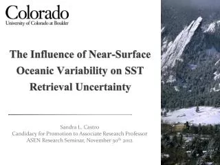
The Influence of Near-Surface Oceanic Variability on SST Retrieval Uncertainty Sandra L. Castro Candidacy for Promotion to Associate Research Professor ASEN Research Seminar, November 30th 2012
There are so many SST products, how do I decide which one to use?
Outline • Motivation • Spatial variability in SSTs at different depths in the water column • Variability in SST due to the presence of the near-surface diurnal thermocline (different from the seasonal thermocline) • Currently funded projects
Outline • Motivation • Spatial variability in SSTs at different depths in the water column • Variability in SST due to the presence of the near-surface diurnal thermocline (different from the seasonal thermocline) • Currently funded projects
The Physics of SST Q net ~ ( -k ) x (r dT/dz ) • This skin layer is generally present, and is ~ 10 µm thick. • It is usually cooler than the water below by ~ 0.3 K
The Near-Surface Thermal Structure of the Ocean IR Radiom Buoys Night Day
1mm -1 m - 5 m Interpreting SST measurements What do radiometers measure and why the near-surface thermal structure of the ocean matters 10μm
Polar-orbiting microwave radiometer Platforms for Measuring SST Geostationary orbit Infrared radiometer Polar-orbitinginfrared radiometer drifting or moored buoy research vessel Argo Floats VOS or SOO
Temperature Measure Processes Uncertainties SST =c0 + Σcj Tb Digital signal, SST Sensor calibration Detector, transducer,amplifier, digitiser TOA radiance (brightnesstemperatures), Tb Atmospheric correction Scattering & absorptionby stratospheric dust Cloud Aerosols Cloud detection Water vapor Precipitation Absorption byWater vapor, etc. eTSkin + (1-e)TSky Water-leavingradiance Surface emissivity effects 10 μm Skin-bulkmodel Skin temperature, TS Thermal microlayer Diurnal thermocline Bulk temperature, Tbulk ? 5 m Processes Affecting SST Measurement Tb TS Tskin 5 cm Diurnal Warming model Tbulk Tbulk
NASA Science Team: SST Error Budget http://www.sstscienceteam.org/white_paper.html • NASA SST Science Team developed White Paper on contributions to the SST uncertainty budget • Diurnal and spatial variability identified as most critical physical processes contributing to the high resolution upper ocean variability
Outline • Motivation • Spatial variability in SSTs at different depths in the water column • Variability in SST due to the presence of the near-surface diurnal thermocline (different from the seasonal thermocline) • Currently funded projects
Do differences in the spatial variability of the thermocline structure of the ocean have an impact on the validation and interpretation of satellite-derived SST products ?
Skin, Bulk or Both? • What do users require? • Tbulk for thermal capacity, deep convection and for existing bulk flux parameterisations. • TS for air-sea interaction processes, better for fluxes • In situ measurements: • Tbulkis conventionally observed • But at what depth? Strictly we should record Tzand z. • May be compromised by DTdiurnal • Shipborne radiometry with sky correction can measure Tskin • Satellite observations • All IR satellites “see” onlyTSkin • TS is precisely defined at the surface. • TS atmospheric algorithms are fundamentally-based • Independent of in situ calibration • Require in situ TS for validation only • Tbulk algorithms have hybrid function • Sensitive to definition of Tbulk • Near-surface SST gradients introduce uncertainties in the SST error budget • DTcool represented as a globally applied bias correction • Need Physical models of DTdiurnal • Require in situ calibration (buoy network)
Traditional Assumption • Since IR satellite retrievals sensitive to the skin temperature, it was believed improvements in regression algorithm accuracy possible through use of in situ skin measurements
Does direct regression of satellite IR brightness temperatures to in situ skin temperatures result in SST-product accuracy improvements over traditional regression retrievals to bulk temperatures?
Approach • We evaluated parallel skin and subsurface MCSST-type models using coincident in situ skin and SST-at-depth measurements from research-quality ship data. • RMS accuracy of skin and SST-at-depth regression equations directly compared
Data: 2003-2005 NOPP Skin SST Satellite IR: 2003-2005 AVHRR/N17 GAC and LAC NAVOCEANO BTs Royal Caribbean EXPLOrer of the seas Skin SST: M-AERI Interferometer (RSMAS) SST-at-depth: Sea-Bird thermometer (SBE-38) @ 2m NOAA R/V Ronald H. Brown Skin SST: CIRIms Radiometer (APL) Sst-at-depth: sea-bird thermometer (SBE-39) @ 2m
Satellite - In situ Matchup Criteria Min Time Mean All Collocation window: 25 km and 4 hours
How much better were the SSTbulk? RMSE differences equivalent to removing an independent error in the bulk SST measurements % Accuracy Improvement
Satellite SST retrievals based on regression models calibrated with in situ bulk SSTs almost always resulted in better accuracies (lower RMSE) than direct skin SST regressions
Can differences in measurement uncertainty and spatial variability explain the lack of accuracy improvement in the skin SST retrievals?
Spatio-Temporal Variability • The issue of the Point-to-Pixel Sampling Characteristics of Remotely Sensed SSTs • Satellite sensors see an “average” value of the radiation emanating from the footprint, whereas in situ instruments measure the emission at single points on the ground • Sub-pixelvariabilitylong acknowledged as source of uncertainty in satellite validation, but magnitude largely unquantified
Approach • To test this hypothesis, we added increasing levels of noise to the SST-at-depth, such that: RMSE bulk SST = RMSE skin SST • Attempt to decompose the supplemental noise into individual contributions from the two effects using Variogram techniques.
Added discrete realizations of white noise processes to SST-at-depth: Build RMSE curve for noise-degraded SST-at-depth. Where the RMSE (skin) intercepts the curve, corresponds to the supplemental noise needed for equivalence in RMSE Note that, for equal number of observations: RMSE SST-at-depth < RMSE SST skin, but RMSE SST skin < RMSE SST emulated buoy
Estimates of Required Noise • Added Noise: • LAC SST:σ ~ O ( 0.09 – 0.14 K ) • GAC SST: σ ~ O (0.14 – 0.17 K )
% Measurement Error & % Spatial Variability? Supplemental Noise: σ ~ O ( 0.1 – 0.2 K )
Instrument Measurement Error • From literature: M-AERI: 0.079°C and CIRIMS: 0.081°C • IR Radiometers: σ~ O(0.08°K) • Thermometers: σ~ O(0.01 K) • Added Noise: σ~ O(0.08°K) • From the data: Empirical distributions for the measurement uncertainty of M-AERI skin SST and coincident SST-at-depth support the required supplemental noise obtained from values reported in the literature!!
Variogram Analysis M-AERI CIRIMS The variogram (Cressie, 1993, Kent et al., 1999) is a means by which it is possible to isolate the individual contributions from the 2 sources of variability, since the behavior at the origin yields an estimate of the measurement error variance, while the slope gives an indication of the changes in natural variability with separation distance.
Method We fitted a linear variogram model by weighted least squares to both skin SST and SST-at-depth with separation distances up to 200 km, and extrapolated to the origin to obtain the variance at zero lag. Measurement Uncertainty M-AERI Spatial Variability
SST Uncertainty Estimates On spatial scales of O(25 km): • Variogram estimates provide strong support to the notion that the combined role of differences in measurement uncertainty and spatial variability between the skin and SST-at-depth account for the range of required subsurface supplemental noise found graphically • Measurement uncertainty estimates are consistent with the noise required to reconcile the accuracy differences between thermometers and IR radiometers (σ~O(0.08 K))
SST Uncertainty Estimates On spatial scales of O(25 km): • Agreement between Variogramestimates and supplemental noise levels provide strong support to the notion that the combined role of differences in measurement uncertainty and spatial variability between the skin and SST-at-depth are responsible for the lack of accuracy improvement in skin-only regressions • Measurement uncertainty estimates are consistent with the noise required to reconcile the accuracy differences between thermometers and IR radiometers (σ~O(0.08 K)) • Measurement uncertainty and spatial variability contribute in equal measure to the overall uncertainty budget
Even if technological advances allowed for better accuracies in the measurements of IR radiometer (say, σ~O(0.01 K)), we still have differences in spatial variability to worry about…Better yet, we need higher accuracy contact thermometers (buoys) and improved atmospheric corrections
Implications • The role of spatial variability in the uncertainty budget arises in part because inadequacies in point-to-pixel comparisons • Sparse radiometric sampling along a single track does not provide full coverage of the spatial variability within the satellite footprint. • The satellite measurement is a spatial average over the IFOV. This integration might be smoothing out the enhanced variability of the skin, making the variability across the pixel more representative of the less variable point measurements of the SST-at-depths • To better understand and quantify these effects, we require increased observations of sub-pixel satellite SST variability. In particular, direct observations of spatial variability as a function of measurement depth are needed.
Outline • Motivation • Vertical variability in SST associated with the near-surface thermal structure of the ocean • Variability in SST associated with the presence of the diurnal thermocline • Current funded projects
The GHRSST Concept • Emphasis on synergy benefits of multi-sensor SST products • In principle, the merging and analysis of complementary satellite and in situ measurements can deliver SST products with enhanced spatial and temporal coverage • Many analyses currently available, but most ignore daytime obs
What is Foundation SST? • Predawn SST • Previous night composite • SST observations at winds greater than 6 m/s Common definitions: Skin SST ΔT cool ΔT diurnal Foundation SST
In recent years, improvements in the accuracy and sampling of geostationary satellites have enabled better characterization of diurnal warming from space • Average difference between MTSAT(skin) and RAMSSA (fnd) for the 1 degree box around 151.5E, 0.5S on 1 Jan 2009
Diurnal Warming Peak Amplitudes • Monthly climatologies of maximum diurnal warming observed from Geostationary MSG/Seviri SSTs for February and June • Previous night composite used as Foundation SST • Amplitudes are small on average but can be significant at low winds
ΔTdiurnal Average effect on fluxes Flux w/ diurnal correction – Flux w/o diurnal correction (W/m2) Clayson and Bogdanoff (2012)
Maximum effect on fluxes (1998 - 2007) Clayson and Bogdanoff (2012)
What is the uncertainty in estimates of diurnal warming as a function of time and depth?
Diurnal Warming Model Validation • APPROACH • Detailed Physical Models • Wick’s Modified Kantha-Clayson • GOTM • COARE • Parametric Models • Castro LUT • CG03 HR Forcing from NWP and Satellite data HR Forcing from Cruises
warming Physical Models of ΔTdiurnal • Wick Modified Kantha-Clayson • Second moment turbulence closure model with enhanced treatment of mixing near the surface • Run with 1-minute resolution and fine vertical grid • Generalized Ocean Turbulence Model (GOTM) • Used 2 different included turbulence schemes • K-epsilon • Mellor-Yamada • Run with 1-minute resolution on same vertical grid • COARE • Warm-layer and cool skin portions of the COARE 3.0 model with included flux computations • Forced with temporal resolution of available forcing data • Solar Penetration Models • 3-band absorption model from COARE (Fairall et al., 1996) • 9-band absorption model from Paulson and Simpson (1981) Wick and Castro
Forcing: Cruise Data • CIRIMS Cruises (Courtesy A. Jessup) • NOAA R/VR. H. Brown cruises from 2003-2005 • HR Skin SSTs from the CIRIMS • Through-the-Hull SST-at-depth (2-3 m) • NOAA/ESRL Cruises (courtesy C. Fairall) • NOAA R/VR. H. Brown cruises from 1992-2000 • Detailed eddy covariance flux measurements • SST-at-depth from the Sea Snake (5-50 cm) Over 300 diurnal warming events!
Real Simulations Skin Validation Sub-skin Validation Models demonstrate ability to reproduce observed warming, but their relative performance varies notably with environmental conditions Wick and Castro