Download
1 / 45
550 likes | 1.57k Views
A digitally reconstructed radiograph (DRR) based computer simulation for optimization of chest radiographs acquired with a CR imaging system. Craig Moore. Introduction - Literature.

E N D
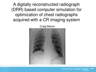
A digitally reconstructed radiograph (DRR) based computer simulation for optimization of chest radiographs acquired with a CR imaging system Craig Moore
Introduction - Literature • Lots of publications have shown that patient anatomy is the limiting factor in the reading normal structures, and detection of lesions (lung nodules) in chest images • Bochud et al 1999 • Samei et al 1999, 2000 • Burgess et al 2001 • Huda et al 2004 • Keelan et al 2004 • Sund et al 2004 • Tingberg et al 2004 • European wide RADIUS chest trial (2005)
Introduction - Literature • Chest radiography is now generally considered to be limited by the projected anatomy • Patient anatomy = anatomical noise So if we want to optimize digital system for chest imaging, vital that anatomical noise is present in the images!!!
Introduction • However, the radiation dose/image quality relationship must not be ignored • Doses must be kelp ALARP • ICRP 2007 • IR(ME)R2000 – (required legally in the UK) • We would therefore want system (quantum) noise present in an image for dose reduction studies
Digitally Reconstructed Radiograph (DRR) • Hypothesis: • Can use CT data of humans to provide realistic anatomy (anatomical noise) • Clinically realistic computerized ‘phantom’ • Simulate the transport of x-rays through the ‘phantom’ and produce a digitally reconstructed radiograph (DRR – a simulation of a conventional 2D x-ray image created from CT data) • Add frequency dependent system noise post DRR calculation • Add radiation scatter post DRR calculation • Validate • Use for optimization studies
1. X-Ray Spectra • X-ray spectra were produced using IPEM Report 78 • Generates spectra at 0.5 keV intervals from 0.5 keV up to tube potential chosen by user. • Data is specified on a central axis 750 mm from source (photons/mm2.mAs) • Fluence is inversely related to square of distance from source, so fluence f(r) at any distance (r) is
2. CT Data Preparation - Filters • CT data used as the ‘patient phantom’ must have as little processing applied as possible, so that CT numbers correspond to the x-ray attenuation properties of the particular tissue • Back-projected CT data is inherently blurred, so processing filter must be applied
2. CT Data Preparation - Filters • Wanted to use filter that gave minimum processing • Discussed this with Philips (Paul Klahr, Physicist) and filter (E) was identified • This filter was therefore used to reconstruct all raw CT data on the scanner prior to transfer to my PC/laptop • Ethics approval obtained for clinical data transfer
3. CT Data Preparation - Noise • CT noise must be characterised by measurement because of reconstruction filter • To characterise noise, used the Radiotherapy Gammex RMI phantom • Contains 17 tissue substitute inserts, the attenuation properties of which mimic the range of those found in humans.
3. CT Data Preparation - Noise • A histogram of pixel values was produced for each insert from a 300 x 300 ROI • The graph shows a histogram of pixel values derived from an ROI placed in the lung insert. • It is clearly a Gaussian distribution with an excellent ‘goodness of fit’. • All other inserts illustrated Gaussian distributions (r2 > 0.97) • As such, noise is Gaussian and is independent of signal strength.
With noise smoothed 3. CT Data Preparation - Noise • Since noise is Gaussian distributed, a technique for removing Gaussian noise from the CT data is required • This can be achieved by using a ‘mean adaptive filter’ (Hilts et al 2004) whilst maintaining edge information. • Mean adaptive filter available in Matlab • All CT data was therefore subject to the filter prior to being used in a DRR calculation.
4. CT Number Conversion to Linear Attenuation Coefficient (LAC) • Prior to DRR calculation, each voxel in the CT data must be converted from its original CT number to linear attenuation coefficient. • Calculated mean CT number of each of the inserts of the Gammex phantom • The elemental composition of each insert is known, and so can calculate LAC of each using the XCOM database • For each photon energy in x-ray beam • Now we know the relationship between CT number (mean) and LAC for each insert. • Derive LACs of all other CT numbers not contained within inserts by interpolation and extrapolation
3D CT data set h (voxel height) w (voxel width) Pencil beam diverging from source to face of voxel phi Distance to patient (DP) theta 5. DRR Calculation • Ray casting method of DRR generation was chosen
5. DRR Calculation • Simulation calculates: • number of photons impinging each voxel in first slice (IPEM 78) • Respective angles (theta and phi) each pencil beam enters voxel • Assumes central axis of pencil beam DOES NOT enter neighbouring voxel in first slice. • This is not the case for subsequent slices
Front face of voxels Central axis of pencil beam is shown by the solid arrow 5. DRR Calculation – Subsequent Slices • Since each pencil beam enters the CT data at angles theta and phi, central axis of beam dose not now impinge centre of voxel in subsequent slices • As such, pencil beam also impinges neighbouring voxels • Need to calculate a weighted LAC based on respective area of beam in the incident, bottom, right and corner voxels
5. DRR Calculation – Subsequent Slices Front face of voxels LACeff = (RATIO_AREAincident x LACincident) + (RATIO_AREAright x LACright) + (RATIO_AREAbottom x LACbottom) + (RATIO_AREAcorner x LACcorner) Central axis of pencil beam is shown by the solid arrow
5. DRR Calculation • This calculation is performed for each slice in the CT data set until the pencil beam exits • The intensity of x-ray photons exiting is calculated with: • Where: • I0 is intensity of photons impinging first slice, • pathlength is the distance traversed by the beam in each voxel • LACeff is the effective LAC for each pencil beam in each slice
6. Energy Absorbed in CR Phosphor • Use the following formula: • Where • is the mass-energy absorption coefficient of phosphor • px is the mass loading of the phosphor (weight per unit area, g/cm2) • Io(E) the incident x-ray photon spectrum • E is the photon energy • Increased absorption of Barium and Iodine k-edge modelled
7. Scatter Addition • X-ray photons scattered in the body that are absorbed in the CR phosphor do not contain clinically useful information • Reduction in contrast • Must add to DRR generated image • DRR model does not include scatter • Need to measure scatter in CR chest images • Use chest portion of RANDO phantom
7. Scatter Addition Primary beam is absorbed in beam stop, only scatter remains in the shadow RANDO CR Cassette Lead stops
7. Scatter Addition • RANDO x-rayed with beam stop array • 50 kVp to 150 kVp in steps of 10 • 2D interpolation used to derive scatter across entire radiograph • Scatter image added to DRR • Warped and then registered to DRR
8. Noise Addition • To add frequency dependent noise to DRR, can use uniform noise image derived for NPS calculation (Bath et al 2005) • Corrected for non-uniformities in DRR • Absolute noise in low dose areas is lower than that in high dose areas • Variance of PVs goes with root of the scaling
8. Noise Addition lung spine diaphragm Corrected noise image Uniform noise image
8. Noise Addition DRR image: 70 kVp, 1 mAs DRR image: 70 kVp, 4 mAs
9. Lung Nodule Simulation • Nodules simulated in CT slices in the lateral pulmanory and hilar regions of the lung • Used the following formula (Li et al 2009): • Where c(r) is the pixel value of the nodule distance r from centre • C is the peak CT number • R is nodule diameter (5 mm) • R is distance pixel is from centre • n is an exponent inversely related to steepness of the contrast profile (dependent on slice thickness)
Human DRR v Human CR DRR CR
10. Validation • Decided to validate with: • Histogram of pixel values • Signal to noise ratios (SNR) • Important because signal and noise affects the visualisation of pathology • Tissue to rib ratios (TRR) • Pixel value ratio of soft tissue to that of rib • Important as rib can distract the Radiologist from detecting pathology
a c b d 10. RANDO Histograms
10. RANDO Histograms • Dynamic range of the DRR generated images typically smaller than that of CR images • This is to be expected because: • we are limited to 17 tissue types in the Gammex phantom (although interpolation performed) • Voxel size = 0.34 x 0.34 x 0.8 mm. This is probably larger than the smaller structures in the body
10. RANDO - SNRs • Good agreement in lung, spine and diaphragm areas of chest • Maximum deviation approx 10% • Mean deviation = 5% • Addition of frequency dependent noise not perfect: • CR system noise is ergodic (changes with time) • Noise added here is a snapshot (and so not ergodic) • However, quantum noise dominates over ‘ergodic noise’ so not such an issue • DQE is NOT constant with dose variation in image
10. RANDO – SNRs with dose reduction As tube current decreases (and therefore x-ray intensity) noise increases. DRR generated images in good agreement with CR images
10. PATIENT - Histograms Typical histogram of average patient DRR Typical histogram of average patient CR image
10. PATIENT - Histograms • Shapes very similar • Min pixel value for 10 CR images = 1712 ± 147 • Min pixel value for 10 DRR images = 1751 ± 133 • Max pixel value for 10 CR images = 2992 ± 128 • Max pixel value for 10 DRR images = 2820 ± 143
11. Validation - TRRs • Good agreement • Within 2% • As tube potential increases TRR decreases • Due to rib attenuating higher percentage in incident photons at lower potentials than soft tissue, thus forcing up TRR
11. Validation - Radiologists • Have told me DRR images contain sufficient clinical data to allow diagnosis and subsequent optimisation
12. W.I.P – Scatter Reduction • All previous simulations included scatter with no anti-scatter/air gap reduction (as per Hull protocol). • Have begun to incorporate into simulation scheme
Conclusions • DRR computer program has been produced that adequately simulates chest radiographs • Anatomical noise simulated by CT data • System noise and scatter successfully added post DRR generation that provides: • SNRs • TRRs • Histograms • in good agreement with those measured in real CR images • Provides us with a tool that can be used by Radiologists to grade image quality with images derived with different x-ray system parameters • WITHOUT THE NEED TO PERFORM REPEAT EXPOSURE ON PATIENTS
Future Work • Find optimum tube potential/dose for chest imaging with CR • Using Radiologist’s scores • Model scatter rejection • Anti-scatter grids • Air gap technique • Simulate large/obese patients and optimize