Download
1 / 61
610 likes | 777 Views
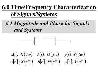
6.0 Time/Frequency Characterization of Signals/Systems 6.1 Magnitude and Phase for Signals and Systems. Signals. : magnitude of each frequency component. : phase of each frequency component. Sinusoidals ( p.68 of 4.0). Signals. Example. See Fig. 3.4, p.188 and Fig. 6.1, p.425 of text.

E N D
6.0 Time/Frequency Characterization • of Signals/Systems • 6.1 Magnitude and Phase for Signals • and Systems
Signals • : magnitude of each frequency component • : phase of each frequency component
Signals • Example See Fig. 3.4, p.188 and Fig. 6.1, p.425 of text • change in phase leads to change in time-domain characteristics • human auditory system is relatively insensitive to phase of sound signals
Signals • Example : pictures as 2-dim signals • most important visual information in edges and regions of high contrast • regions of max/min intensity are where different frequency components are in phase See Fig. 6.2, p.426~427 of text
Systems • : scaling of different frequency components • : phase shift of different frequency • components
Systems • Linear Phase (phase shift linear in frequency) means • constant delay for all frequency components • slope of the phase function in frequency is the delay • a nonlinear phase may be decomposed into a linear part plus a nonlinear part
Time Shift (P.19 of 4.0) • Time Shift • linear phase shift (linear in frequency) with amplitude unchanged
Time Shift (P.20 of 4.0)
Systems • Group Delay at frequency ω • common delay for frequencies near ω
Systems • Examples • See Fig. 6.5, p.434 of text • Dispersion : different frequency components delayed • by different intervals • later parts of the impulse response oscillates at near 50Hz • Group delay/magnitude function for Bell System telephone lines See Fig. 6.6, p.435 of text
Systems • Bode Plots • Discrete-time Case • ω not in log scale, finite within [ -, ] • Condition for Distortionless • Constant magnitude plus linear phase in signal band
6.2 Filtering Ideal Filters • Low pass Filters as an example • Continuous-time or Discrete-time • See Figs. 6.10, 6.12, pp.440,442 of text • mainlobe, sidelobe, mainlobe width
Filtering of Signals (p.55 of 4.0) 1 1 1 0 0 0
Ideal Filters • Low pass Filters as an example • with a linear phase or constant delay • See Figs. 6.11, 6.13, pp.441,442 of text • causality issue • implementation issues
Realizable Lowpass Filter (p.58 of 4.0) 0 0 0
Ideal Filters • Low pass Filters as an example • step response See Fig. 6.14, p.443 of text overshoot, oscillatory behavior, rise time
Nonideal Filters • Frequency Domain Specification • (Lowpass as an example) • δ1(passband ripple), δ2(stopband ripple) • ωp(passband edge), ωs(stopband edge) • ωs - ωp(transition band) • phase characteristics magnitude characteristics See Fig. 6.16, p.445 of text
δ1(passband ripple), δ2(stopband ripple) • ωp(passband edge), ωs(stopband edge) • ωs - ωp(transition band) magnitude characteristics
Nonideal Filters • Time Domain Behavior : step response • tr(rise time), δ(ripple), ∆(overshoot) • ωr(ringing frequency), ts(settling time) See Fig. 6.17, p.446 of text
tr(rise time), δ(ripple), ∆(overshoot) • ωr(ringing frequency), ts(settling time)
Nonideal Filters • Example: tradeoff between transition band width • (frequency domain) and settling time (time domain) See Fig. 6.18, p.447 of text
Nonideal Filters • Examples • linear phase • See Figs. 6.35, 6.36, pp.478,479 of text • A narrower passband requires longer impulse response
Nonideal Filters • Examples • A more general form • See Figs. 6.37, 6.38, p.480,481 of text • A truncated impulse response for ideal lowpass filter gives much sharper transition • See Figs. 6.39, p.482 of text • very sharp transition is possible
Nonideal Filters • To make a FIR filter causal
6.3 First/Second-Order Systems • Described by Differential/Difference • Equations • Higher-order systems can usually be represented as combinations of 1st/2nd-order systems • Continuous-time Systems by Differential Equations • first-order • second-order See Fig. 6.21, p.451 of text
Discrete-time Systems by Differential Equations • first-order See Fig. 6.26, 27, 28, p.462, 463, 464, 465 of text • second-order
First-order Discrete-time system (P.461 of text) y[n] x[n] D a y[n-1]