Download
1 / 21
210 likes | 358 Views
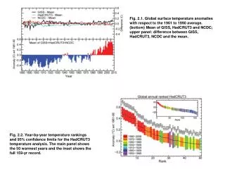
Fig. 2.1. Global surface temperature anomalies with respect to the 1961 to 1990 average. (bottom) Mean of GISS, HadCRUT3 and NCDC; upper panel: difference between GISS, HadCRUT3, NCDC and the mean.

E N D
Fig. 2.1. Global surface temperature anomalies with respect to the 1961 to 1990 average. (bottom) Mean of GISS, HadCRUT3 and NCDC; upper panel: difference between GISS, HadCRUT3, NCDC and the mean. Fig. 2.2. Year-by-year temperature rankings and 95% confidence limits for the HadCRUT3 temperature analysis. The main panel shows the 50 warmest years and the inset shows the full 159-yr record.
Plate 2.1. Global annual anomaly maps for those variables for which it was possible to create a meaningful anomaly estimate. Climatologies differ among variables, but spatial patterns should largely dominate over choices of climatology period. Dataset sources and climatologies are given in the form (dataset name/data source, start year–end year) for each variable. See relevant section text and figures for more details. Lower stratospheric temperature (RSS MSU 1981–90); lower tropospheric temperature (UAH MSU 1981–90); surface temperature (NCDC 1961–90); cloud cover (PATMOS-x 1982–2008); total column water vapor (SSM/I/GPS 1997–2008); precipitation (RSS/GHCN 1989–2008); mean sea level pressure (HadSLP2r 1961–90); wind speed (SSM/I1988–2007); total column ozone (annual mean global total ozone anomaly for 2008 from SCIAMACHY. The annual mean anomalies were calculated from 1° × 1.25° gridded monthly data after removing the seasonal mean calculated from GOME (1996–2003) and SCIAMACHY (2003–07)]; vegetation condition [annual FAPAR anomalies relative to Jan 1998 to Dec 2008 from monthly FAPAR products at 0.5° × 0.5° [derived from SeaWiFS (NASA) and MERIS (ESA) data].
Fig. 2.3. HadCRUT3 monthly average temperature anomalies by latitude for the period 1850 to 2008. The data have been smoothed in space and time using a 1:2:1 filter. White areas indicate missing data. Fig. 2.4. Global mean lower tropospheric temperature (1958–2008) from multiple datasets, including five radiosonde datasets (HadAT, IUK, RAOBCORE, RATPAC, and RICH) and two satellite MSU datasets (RSS, UAH). All time series are for the layer sampled by MSU retrieval 2LT, spanning 0–8 km in altitude. Black curve is the average of all available radiosonde datasets, and the colored curves show differences between individual datasets and this average. References for the radiosonde datasets are Thorne et al. 2005b, Sherwood et al. 2008, Haimberger 2007, Free et al. 2005, and Haimberger et al. 2008; and for the MSU dataset
Fig. 2.5. Zonal mean lower tropospheric temperature anomalies (1979–2008) with respect to the 1979–88 mean. Anomalies based on MSU Channel 2LTdata, as processed by RSS (Mears and Wentz 2009a). Fig. 2.6. As Fig. 2.4. but all time series are for the layer sampled by MSU channel 4, spanning 10–25 km in altitude, with a peak near 18 km. Additional dataset is STAR (Zou et al. 2008) and RSS Channel 4 is described in Mears and Wentz (2009b).
Fig. 2.7. As Fig. 2.5 but for the lower stratospheric channel (Mears and Wentz 2009b). Fig. 2.8. Global mean temperature changes over the last decade in context. (a) Monthly global mean temperature anomalies (with respect to 1961–90 climatology) since 1975, derived from the combined land and ocean temperature dataset HadCRUT3 (gray curve). (top blue curve) The global mean after the effect of ENSO that has been subtracted is also shown, along with (bottom blue curve, offset by 0.5°C) the ENSO contribution itself. Least squares linear trends in the ENSO and ENSO-removed components for 1999–2008 and their two std dev uncertainties are shown in orange. (b) ENSO-adjusted global mean temperature changes to 2008 as a function of starting year for HadCRUT3, GISS dataset (Hansen et al. 2001) and the NCDC dataset (Smith et al. 2008) (dots). Mean changes over all similar-length periods in the twenty-first century climate model simulations are shown in black, bracketed by the 70%, 90%, and 95% intervals of the range of trends (gray curves). (c) Distribution of 1999–2008 trends in HadCRUT3 (°C decade–1). Black squares indicate where the trends are inconsistent at the two std dev level with trends in 17 simulated decades (see text).
Fig. 2.9. 2008 annual mean TCWV (mm) at 252 stations (colored circles) and 308 stations (denoted by an asterisk) that have data in 2008, but not enough to calculate an annual mean. Fig. 2.10. Anomaly time series of TCWV both from SSM/I and from an average of GPS stations. The time series have been smoothed to remove variability on time scales shorter than 6 months. A linear fit to the SSM/I data is also shown, indicating an increasing trend in water vapor over the 1988–2008 period.
Fig. 2.11. Time–latitude plot of TCWV anomaly calculated using a reference period of 1988–2007. The data have been smoothed in the time direction to remove variability on time scales shorter than 4 months. Fig. 2.12. (a) Annual global land surface precipitation anomalies (mm) over the period 1901–2008 from the GHCN dataset (Vose et al. 1992). Precipitation anomalies were calculated with respect to 1981–2000 (Trenberth et al. 2007): green bars are positive anomalies, yellow bars are negative anomalies, and red bar is 2008 anomaly. Smoothed GHCN and CRU (v.3) annual values were created using a 13-point binomial filter. (b) Time series of the difference between the smoothed GHCN annual anomalies and annual anomalies over global land areas from five different global precipitation datasets for the period 1951–2008: CRU v.3, Chen et al. (2002), GPCP, and two from the GPCC (VasClimOand Full v.3). (c) Ocean precipitation anomalies relative to the period 1988–2008. Averages are for the global ocean between 60°S and 60°N latitude using a common definition of “ocean.” The annual cycle has been removed and the time series have been low-pass filtered by convolution using a Gaussian distribution, with 4-month width at half-peak power. Note that the RSS data are available through all of 2008, while GPCP and CMAP data are available through Apr and Jul 2008, respectively. The inset gives the 1988–2008 mean (mm yr−1) and the linear trend (mm yr−1 decade−1) with the 95% confidence interval. Straight lines denote the linear trends, and the confidence interval is estimated based on deviations from the linear fit and does not incorporate a particular dataset’s “error.”
Fig. 2.13. Trends in annual precipitation calculated from the GHCN monthly dataset for two different time periods: (a) 1901–2008 (% change century−1) and (b) 1989–2008 (% change decade−1). Calculation of grid cell trends required at least two-thirds (66%) of the years without missing data during each of the two periods analyzed. Fig. 2.14. (a) Time–latitude plot of GHCN annual land precipitation in terms of the % departure from 1989 to 2000 base-period means, with zonal means determined over 5°-latitude bands covering the period 1901–2008. Gray shading at higher latitudes in the early twentieth century is due to a lack of data south of 40°S and north of 75°N. (b) Same as (a) but for the RSS satellite record era. (c–e) Time–latitude section of precipitation anomalies (mm yr−1) averaged over the (c) Atlantic, (d) Pacific, and (e) Indian Ocean basins as observed by the RSS monthly averaged dataset. Anomalies were calculated using the 1988–2008 base period by removing the latitude-dependent annual cycle.
Fig. 2.15. Time–longitude section of precipitation anomaly averaged over the tropical ocean (5°S to 5°N) as observed by the RSS monthly averaged dataset. Anomalies were determined using the 1988–2008 base period by removing the longitude-dependent annual cycle. Missing areas are the results of land masks: between 10° and 40°E are due to Africa, the areas near 100° and 115°E are due to Sumatra and Borneo, and the areas between 280° and 310°E are due to South America. Fig. 2.16. Global map of daily precipitation extremes observed in 2008 from the GHCN dataset. The plotted values are the average of the top five largest daily precipitation events (mm) at each station.
Fig. 2.17. Anomalies of monthly snow cover extent over Northern Hemisphere lands (including Greenland) between Nov 1966 and Dec 2008. Anomalies are calculated from NOAAsnow maps. Mean hemispheric snow extent is 25.5 million km2 for the full period of record. Monthly means for the period of record are used for nine missing months between 1968 and 1971 to create a continuous series of running means. Missing months fall between Jun and Oct; no winter months are missing. Fig. 2.18. Seasonal snow cover extent over Northern Hemisphere lands (including Greenland) between winter (Dec–Feb) 1966/67 and fall (Sep–Nov) 2008. Calculated from NOAA snow maps.
Fig. 2.19. (a) Monthly zonal average PATMOS-x anomalies of high cloud cover (cloud top pressure < 440 hPa) in 2008, relative to 2003–08 climatology based on retrievals from the NOAA-16 and NOAA-18 satellites. The 2003–08 reference period is chosen to match that of MODIS (b) to facilitate comparison. (b) Same as (a) but for MODIS (cloud top pressure < 440 hPa) based on retrievals from the Aqua and Terra satellites. Fig. 2.20. Anomalies of monthly cloud amount between Jan 1971 and Dec 2008 taken from four datasets. The thick solid lines represent smoothing with a boxcar filter with a 2-yr window. There are 6 months missing from the PATMOS-x time series between Jan 1985 and Feb 1991, as well as a gap from Jan 1994 to Feb 1995.
Fig. 2.21. Estimates for 2007 of (a) runoff and (b) its anomaly based on outputs from a hydrometeorological model utilizing GPCP precipitation measurements. Fig. 2.22. The SOI for (a) 1900 to present and (b) from 2000 to 2008 relative to the 1876 to 2008 base period.
Fig. 2.23. (a) The annual historical instrumental [Ponta Delgada (Azores) minus Stykkisholmur (Iceland), normalized] NAO series from the mid-1860s to present (blue); the 21-point binomial filter run through the data three times (red). The green bar shows the average for the 2007/08 boreal winter. (b) Standardized 3-month running-mean value of the SAM or AAO index from 1979. The loading pattern of the SAM/AAO is defined as the leading mode of EOF analysis of monthly mean 700-hPa height during the 1979–2000 period. The monthly SAM/AAO index is constructed by projecting the monthly mean 700-hPa height anomalies onto the leading EOF mode. The resulting time series are normalized by the std dev of the monthly index (1979–2000 base period). Source: www.cpc.ncep.noaa.gov/products/precip/CWlink/daily_ao_index/aao/aao.shtml. Fig. 2.24. Surface wind speed anomalies averaged over the global ice-free oceans. The time series has been smoothed to remove variability on time scales shorter than 4 months. The reference period for the SSM/I measurements is 1988–2007. For the QuikSCAT measurements the reference period is 2000–07, with the mean adjusted to match the SSM/I anomalies for the 2000–07 period.
Fig. 2.25. Surface wind speed anomalies by latitude (reference period 1988–2007) over the ice-free oceans. The data have been smoothed in time to remove variability on time scales shorter than 4 months. Fig. 2.26. Time series of global monthly mean deseasonalized anomalies of TOA Earth Radiation Budget for longwave (red line), shortwave (blue line), and net radiation (green line) from Mar 2000 to Dec 2008. Anomaly is computed relative to the calendar month climatology derived for the Mar 2000 to Dec 2008 period. The shaded green/yellow/pink area of the figure indicates the portion of the time series that is constructed using the CERES EBAF (Mar 2000 to Oct 2005)/CERES ERBE-like (Nov 2005 to Aug 2007)/FLASHFlux (Sep 2007 to Dec 2008) dataset, respectively. All three datasets are derived directly from CERES measurements. EBAF has been renormalized so that globally averaged top-of-atmosphere net radiation from 2000 to 2005 is consistent with ocean heat storage value (Willis et al. 2004; Hansen et al. 2005; Wong et al. 2006). The green (EBAF) and yellow (ERBE-like) shading indicate high-quality climate data with in-depth on-orbit instrument stability analysis. The pink shading (FLASHFlux) indicates preliminary climate data with possible instrument stability artifacts. Mean differences among datasets were removed using available overlapping data, and the combined ERBE time series was anchored to the absolute value of EBAF before deseasonalization.
Fig. 2.27. CO2 dry air mole fractions (top: NOAAESRL) and δ 13C in CO2 (bottom: University of Colorado, INSTAAR, courtesy James White) from weekly samples at Cape Kumukahi, HI. Fig. 2.28. (a) CO2 monthly mean mole fractions determined from NOAAESRL observatories at Barrow, AK; Mauna Loa, HI; American Samoa; and South Pole, part of the larger global carbon-cycle monitoring network shown in (b). 2008 results are preliminary. Data are courtesy of Kirk Thoning, NOAAESRL. Current CO2 trends at MLO are available at www.esrl.noaa.gov/gmd/ccgg/trends/. Additional plots can be found at www.esrl.noaa.gov/gmd/ccgg/iadv/ and www.esrl.noaa.gov/gmd/Photo_Gallery/GMD_Figures/ccgg_figures/.
Fig. 2.29. Changes in global mean tropospheric mixing ratios (ppt, or pmol mol−1) of the most abundant CFCs, HCFCs, HFCs, chlorinated solvents, and brominated gases. The middle right-hand panel shows secular changes in atmospheric equivalent chlorine (EECl; ppb or nmol mol−1), which is an estimate of the ozone-depleting power of these atmospheric halocarbons. EECl is derived from observed mixing ratios of ozone-depleting gases appearing in the other four panels, and it is derived from the sum of [Cl + (Br×60)] contained in these gases. The bottom shows the recent changes in EESC observed by the NOAA/GMD global network relative to the secular changes observed in the past, including the level observed in 1980 when the ozone hole was first observed, and a projected future. The Ozone Depleting Gas Index for midlatitudes is derived (right-hand axis) from rescaling EESC. EESC is derived from EECl by simply adding 3 yr to the time axis to represent the lag associated with mixing air from the troposphere to the middle stratosphere, where the ozone layer resides [Source: Montzka et al. (1996, 1999.)] Fig. 2.30. The NOAA AGGI shows radiative forcing relative to 1750, of all the long-lived greenhouse gases indexed to 1 for the year 1990. Since 1990, radiative forcing from greenhouse gases has increased 24%.
Fig. 2.31. (top) Global monthly means along with estimates for the linear growth rate of atmospheric nitrous oxide (N2O, red) in ppb and sulfur hexafluoride (SF6, blue) in ppt from the NOAA/ESRL halocarbon network. (bottom) Instantaneous growth rate of N2Oand SF6 using a smoothing algorithm with a 2-yr filter; note the rapid rise of the atmospheric SF6 growth rate after 2003. Atmospheric data for N2O prior to 1989 and for SF6 prior to 1999 were analyzed from flasks instead of continuously operating instruments at NOAA/ESRL baseline observatories. Fig. 2.32. Annual mean total aerosol optical depth derived from the MODIS Aqua sensor for (a) 2007, (b) 2008. (c) The anthropogenic aerosol optical depth derived from MODIS aerosol optical depths and fine-mode fractions for 2008, following Bellouin et al. (2008). Missing data areas are white.
Fig. 2.33. (a) The change in aerosol optical depth simulated by the Met Office HadGEM1 over the period 1980 to 2000. Blue and gray represent a decrease in aerosol optical depths over Europe and the eastern United States due to more stringent emission controls, while red and yellow represent emissions from increasingly industrialized regions. (b) The modeled change in sunlight received at the surface (W m−2) for the same period—“brightening” is shown in yellow/orange, while “dimming” is shown in the blue colors. Fig. 2.34. Time series of SBUV/TOMS/OMI (black), GOME (red), and SCIAMACHY (blue) total ozone in the bands 50°–90°N in Mar, 20°S–20°N (annual mean), and 50°–90°S in Oct. Anomalies were calculated from area-weighted monthly mean zonal mean data in 5° latitude steps by removing the seasonal mean from the period 1979–89.
Fig. 2.35. Time variation (1979–2008) of zonally averaged total ozone anomalies. Anomalies are based on the merged SBUV/TOMS/OMI up to Jun 1995 (Frith et al. 2004), GOME from Jul 1995 to May 2003, and SCIAMACHY data from Jun 2003 to Dec 2008 (Weber et al. 2007). Fig. 2.36. (a) The mean annual mass balance (mm water equivalent) of 30 WGMS reference glaciers, 1980–2007. (b) The mean cumulative mass balance for the 30 reference glaciers and all monitored glaciers. The dashed line is for subset of 30 reference glaciers because not all 30 glaciers have final data for the last few years.
Fig. 2.37. Global land cover at the turn of the millennium: 22 land-cover classes, legend compatible with the FAOL and Cover Classification System (Di Gregorio and Jansen 2000). Projection Interrupted Goode Homolosine Classification derived from daily SPOTVGT satellite observations, 1 × 1 km grid cell, between Nov 1999 and Dec 2000. Map and independent reference data agree 68.6% of the time (Mayaux et al. 2006). Twenty-two percent of the misclassified areas occur in the mixed classes (e.g., some areas known from reference data to be broad-leaved deciduous forest have been mapped as mixed forest).
Fig. 2.38. Conversion of natural vegetation to agriculture and reversion of agriculture to natural vegetation between 1975 and 2000 for Africa; rates range from −1.96% to 35.5% Fig. 2.39. Zonal-average FAPAR anomalies 1998–2008. Values range from −0.06 to 0.06.