Download
1 / 31
310 likes | 447 Views
Recommended dataset of primary and secondary aerosol emissions for use in AEROCOM. Contributors: Frank Dentener, Julian Wilson, Luisa Marelli, JP Putaud (IES, JRC, Italy) Tami Bond (U. Washington, USA) Judith Hoelzemann, Stephan Kinne (MPI Hamburg, Germany)

E N D
Recommended dataset of primary and secondary aerosol emissions for use in AEROCOM Contributors: Frank Dentener, Julian Wilson, Luisa Marelli, JP Putaud (IES, JRC, Italy) Tami Bond (U. Washington, USA) Judith Hoelzemann, Stephan Kinne (MPI Hamburg, Germany) Sylvia Generoso, Christiane Textor, Michael Schulz (CEA, FRANCE) Guido v.d. Werf (NASA USA) Sunling Gong (ARQM Met Service Canada) Paul Ginoux (NASA, USA) Janusz Cofala (IIASA, Austria) O. Boucher (LOA, France) Date: 13.11.2003
Goal: • To provide a single recommended data set for the 2000 of anthropogenic aerosol and precursor gases. Recommendations on aerosol size distributions of primary emissions and temporal distributions. Basic descriptions of datasets. • The following datasets are provided: • Large scale biomass burning OC/EC/SO2 • Fossil fuel/biofuel related OC/EC emissions • SO2 emissions, fossil fuel, fraction emitted as sulfate • Seasalt emissions size resolved • Dust emissions size resolved • DMS emissions • SOA ‘effective’ emissions • Height of emissions • For datasets needed e.g. for ‘full chemistry’ simulations it is recommended to use EDGAR 3.2 1995 (e.g. for NOx/ anthropogenic NMHC). http://arch.rivm.nl/env/int/coredata/edgar • We do not give specific recommendations for oxidant fields.
Large scale biomass burning: POM/EC/SO2 • GFED (GLOBAL EMISSIONS DATA BASE VERSION1) • 2000. • http://www.gps.caltech.edu/~jimr/randerson.html • Van der Werf et al., Carbon emissions from fires in tropical and Tropical ecosystems, Global Change Biology, 2003. • (includes ‘large’ agricultural fires) • Global emissions total [Tg]: • POM 34.7 Tg Particulate organic matter (or 24.8 Tg OC-C) • EC 3.04 Tg C- SO2 4.11 Tg SO2 • Note: in AEROCOM we use Particulate Organic Matter (POM) rather than OC. • Compare to literature: • T. Bond POM-34.6, OC 25.05 -BC 3.32 ‘open burning’ category • S. Generoso: 29.3 POM- BC 3.33 (ACP, 2003) • Compare: SO2 to EDGAR3.2 (deforestation+savannah+mid latitude • burning): 2.7 Tg SO2 (changed emissions factors)
Fossil fuel related emissions SPEW: A technology based global inventory of black and organic \carbon emissions from combustion. Base 1996. Tami Bond: A technology based global inventory of black and organic carbon emissions from combustion, revised to JGR, 2003. totals [Tg EC-C, OC-C, or POM per year]: BC OC* POM fossil 3.04 2.44 5.13 biofuel 1.63 6.50 19.0 (open fires 3.32 25.08 34.6)** Total 7.99 34.02 58.73 This is 35 % lower than previous inventory, which was based on 1984 statistics * Old version of data set before resubmission of paper. ** For large scale burning we use GFED
Comparison of EC emissions SPEW, open burning GFED SPEW/BOND biofuel open fire fossil fuel OPEN OCEAN 1.42e+06 7.80e+05 2.93e+07 CANADA 8.08e+06 5.28e+07 3.57e+07 USA 6.33e+07 6.28e+07 2.92e+08LATIN AMER 1.08e+08 9.10e+08 3.04e+08 AFRICA 3.48e+08 1.47e+09 1.25e+08OECD EUROP 2.96e+07 5.26e+07 2.78e+08EASTERN EU 3.36e+07 6.40e+06 9.88e+07CIS (FORME 1.77e+07 1.01e+08 1.67e+08MIDDLE EAS 1.73e+07 2.03e+07 1.32e+08INDIA REGI 4.27e+08 1.64e+08 1.86e+08CHINA REGI 4.54e+08 1.87e+08 1.01e+09EAST ASIA 1.23e+08 1.28e+08 1.99e+08OCEANIA 4.28e+06 1.64e+08 2.94e+07JAPAN 3.60e+04 2.51e+06 1.56e+08 WORLD 1.63e+09 3.32e+09 3.04e+09 GFED Open Fire 0.00e+008.75e+066.78e+078.63e+081.54e+096.42e+066.21e+068.31e+073.74e+058.83e+076.39e+071.14e+082.13e+087.97e+053.06e+09 Note for Aerocom we use GFED open fire
BC-inventories for open biomass burning: GWEM (JH,Hoelzemann), Generoso (SG), and GFED (2000)
POM biofuel open fossilOPEN OCEAN 7.37e+06 8.17e+06 1.22e+08CANADA 6.15e+07 8.64e+08 2.90e+07USA 4.82e+08 1.17e+09 2.15e+08LATIN AMER 7.25e+08 9.40e+09 4.17e+08AFRICA 1.86e+09 1.47e+10 2.11e+08OECD EUROP 2.24e+08 8.94e+08 1.98e+08EASTERN EU 2.84e+08 4.91e+07 1.06e+08CIS (FORME 1.45e+08 1.71e+09 1.69e+08MIDDLE EAS 7.60e+07 1.71e+08 2.67e+08INDIA REGI 2.28e+09 1.26e+09 1.49e+08CHINA REGI 2.27e+09 1.49e+09 9.64e+08EAST ASIA 6.55e+08 1.28e+09 2.40e+08OCEANIA 2.01e+07 1.55e+09 2.17e+07JAPAN 1.97e+05 1.14e+07 9.35e+07WORLD 9.09e+09 3.46e+10 3.20e+09 GFED 2000 Open burning 0.00e+001.81e+081.11e+099.81e+091.61e+101.05e+081.21e+081.81e+094.76e+069.33e+088.25e+081.23e+092.41e+091.23e+073.47e+10 Note open burning SPEW not used in AEROCOM.
Comparison of POM (using conversion factor OC-POM of 1.4 2000)
SO2 emissions (see also Volcano and SO4 SO4 emissions): Janusz Cofala (IIASA, manuscript in prep. 2003): Country based SO2 emissions for the 2000, using RAINS, gridded according the EDGAR3.2 1995 distribution (FD). Ships 2000 use 1.5 % per increase since 1995. A flat percentage of 2.5 % of all SO2 is emitted as primary SO4 (see sulfate Emissions). Totals: Tg SO2 Tg S Powerplants 48.4 24.2 Industry 39.2 19.6 Domestic 9.5 4.77 RoadTransport 1.9 0.96 Off-road 1.6 0.78 Biomass burning (GFED) 4.1 2.06 International_Shipping 7.7 3.86 Volcanoes 29.2 14.6 Total 141.7 70.9 Emitted as SO2 138.2 69.1 Emitted as SO4 5.3 (Tg SO4!) 1.8
Some cross-checks: Total Tg SO2 1990 1995 2000 IIASA+GFED+SHIP 131.6 118.5 112.5 EDGAR3.2 154.9 141.19 - Decrease between 1990 and 1995 similar between EDGAR and IIASA; but in general IIASA 15 % lower than EDGAR REGIONAL ESTIMATES: Tg SO2 regio Domestic_2 Industry_2 Intern. ship Off-road_2 Powerplant RoadTransp GFED_SO2 OPEN OCEAN 0.00e+00 0.00e+00 5.05e+09 0.00e+00 0.00e+00 0.00e+00 CANADA 7.16e+07 1.19e+09 2.90e+07 5.30e+07 5.44e+08 1.35e+07 USA 3.11e+08 3.12e+09 8.45e+07 1.11e+08 1.25e+10 1.67e+08 LATIN AMER 1.96e+08 2.96e+09 1.71e+08 1.99e+08 2.37e+09 2.98e+08 AFRICA 3.95e+08 1.50e+09 2.54e+08 6.90e+07 2.56e+09 1.79e+08 OECD EUROP 4.42e+08 2.05e+09 1.64e+09 1.89e+08 3.47e+09 1.43e+08 EASTERN EU 6.70e+08 1.01e+09 7.73e+07 3.63e+07 4.20e+09 2.96e+07 CIS (FORME 1.16e+09 3.99e+09 0.00e+00 1.23e+08 5.61e+09 5.82e+07 MIDDLE EAS 5.17e+08 2.44e+09 2.32e+08 6.30e+07 2.80e+09 2.48e+08 INDIA REGI 5.95e+08 2.90e+09 1.93e+07 1.34e+08 3.49e+09 4.36e+08 CHINA REGI 4.76e+09 1.47e+10 1.93e+07 3.45e+08 8.73e+09 1.24e+08 EAST ASIA 3.50e+08 2.08e+09 1.26e+08 1.55e+08 1.09e+09 1.52e+08 OCEANIA 8.30e+06 8.06e+08 7.24e+06 4.29e+07 8.50e+08 3.67e+07 JAPAN 6.76e+07 4.79e+08 4.10e+07 4.09e+07 2.45e+08 3.71e+07 WORLD 9.55e+09 3.92e+10 7.75e+09 1.56e+09 4.84e+10 1.92e+09 total world 2000: 112.5 0.00e+001.50e+071.11e+089.98e+082.20e+091.05e+071.06e+071.47e+085.71e+051.04e+087.35e+071.13e+083.22e+081.29e+064.11e+09
VOLCANO SO2: Since there are no specific data sets for the 2000, we use a combination of the GEIA datasets on Volcano emissions. http://www.geiacenter.org/, Andres and Kasgnoc, JGR,1998 (http://www.igac.noaa.gov/newsletter/22/sulfur.php ) supplemented with a dataset on explosive volcanoes We provide 2 datasets: SO2 emissions from continuous erupting volcanoes (continuous_volc.nc, And eruptive_volc.nc) We give a short summary of Table 6 and Table 1 of the first and the second website given above, respectively: specie Tg S/a SO2 6.70 (of which 4.7 contineous and 2.0 explosive degassing) H2S 2.6 CS2 0.25 OCS 0.16 SO4 0.15 part S 0.081 other S 0.54 SUM 10.4 (SUM of non-SO2~3.7 of which most important H2S )The annual long-time average emission of sulfur recommend by GEIA of 10.4 Tg/a S is for various reasons considered to be an underestimate, see the following publications: Graf, H.-F., B. Langmann, and J. Feichter, The contribution of Earth degassing to the atmospheric sulfur budget, Chemical Geology 147, 131-145, 1998. Textor, C., H.-F. Graf, C. Timmreck, and A. Robock, Emissions from volcanoes, Chapter 7 of Emissions of Chemical Compounds and Aerosols in the Atmosphere, Claire Granier, Claire Reeves, and Paulo Artaxo, Eds., (Kluwer, Dordrecht), in press 2003.
Therefore we multiply the GEIA continuous SO2 emissions to account for all non-SO2 sulfur species by a factor of 1.5 to get 12.6 TgS/a. This amount is be emitted continuously in the models in the form of 25.2Tg SO2/a. (contSO2+nonSO2)*1.5 TgS/a = (4.7+3.7) *1.5 TgS/a = 12.6 TgS/a = 25.2 TgSO2/a These emissions should be distributed in the model layers between the volcano height h und 1/3 below this height to account for degassing at the flanks of the models. These heights are contained in the datafile. For explosive emissions observed by TOMS and by other techniques (called 'sporadically erupting' by GEIA) the GEIA Table gives a long-term average emission of 2TgS/a=4TgSO2/a. This should be emitted continuously to account for the fact that explosive volcanoes emit only about 1/3 of their emissions during the paroxysmal phases, but 2/3 pre- and post eruptive. The GEIA data set contains only very few locations for explosive volcanoes, and we believe that these are not representative for the regions of active explosive volcanism. For this reason, we take the locations of explosive volcanoes which had been active during the last 100 years from Halmer et al. [2002]: Halmer, M. M., H.-U. Schmincke, and H.-F. Graf , The annual volcanic gas input into the atmosphere, in particular into the stratosphere: a global data set for the past 100 years, Journal of Volcanology and Geothermal Research, 115, 511-528, 2002. We homogeneously distribute the 4Tg SO2/a suggested by the GEIA data for explosive set on these appr. 370 volcanoes. To account for the explosivity of the eruptions, the SO2 should be emitted at a height interval reaching from 500m to 1500m above the mountain height. These heights are included in the data file. Our correction leads to a total volcanic sulfur emission of 25.2 TgSO2/a from continuously degassing volcanoes + 4 TgSO2/a from explosive volcanoes = 29.2 TgSO2/a all volcanoes = 14.6 TgS /a
Primary SO4 emissions: A flat rate of 2.5 % of all SO2 emissions are considered to be in the form of primary sulfate. Literature values range between 1-5 %. Industrial and power plant emissions are assumed to be associated with Coarse mode fly-ash. All other emissions are assumed to be in the aitken and accumulation mode. Note that no separate data files are Given for SO4 emissions. The SO4 emission are 5.3 Tg SO4 or 1.8 Tg S/yr. Note that we do not provide separate files for the SO4 primary Emissions.
SOA (Secondary organic aerosol): At present it is not possible to describe SOA production in a simplified manner. Estimates of global annual production range from 10-60 Tg OA p/a. Most recent estimates (e.g. overview in Tsigaridis et al., ACPD 2003) tend to the lower end. In this work we consider that a fixed fraction of 15 % of the natural terpene emissions forms SOA. This SOA is formed on time scales of a few hours and less and can be treated as ‘direct’ emissions SOA emissions of 19.11 Tg POM per year. (file SOA.ncf). These pseudo-SOA emissions condense on existing pre-existing aerosol. Time resolution is 12 months.
PRIMARY AEROSOL EMISSIONS SIZE DISTRIBUTIONS (I) Seasalt emissions: Original dataset of S. Gong (20 bins) Gong, S.L., and L.A. Barrie, Simulating the Impact of Sea-salt on Global nss-Sulphate Aerosols, J. Geophys. Res., 108 (in press), 2003.Gong, S.L., L.B. Barrie, and M. Lazare, CAM: A Size Segregated Simulation of Atmospheric Aerosol Processes for Climate and Air Quality Models 2. Global sea-salt aerosol and its budgets, J. Geophys. Res., 107, 2002. The original numbers submitted by S. Gong are as follows: Total amounts are 96.3 and 23100 Tg of sub and supermicron seasalt aerosol emissions Units are kg dry mass.Compare to IPCC-TAR recommend 10-100 Tg/year. kg and fraction Submicron Supermicron Global Total Sub/Total Sup/Total Jan 7.81E+09 1.87E+12 1.88E+12 4.16E-03 9.97E-01 Feb 8.10E+09 1.94E+12 1.95E+12 4.16E-03 9.97E-01 Mar 8.45E+09 2.02E+12 2.03E+12 4.16E-03 9.97E-01 Apr 7.85E+09 1.88E+12 1.89E+12 4.15E-03 9.96E-01 May 8.16E+09 1.96E+12 1.96E+12 4.16E-03 9.97E-01 Jun 7.84E+09 1.88E+12 1.89E+12 4.15E-03 9.97E-01 Jul 8.34E+09 2.00E+12 2.00E+12 4.16E-03 9.97E-01 Aug 8.45E+09 2.02E+12 2.03E+12 4.16E-03 9.97E-01 Sep 7.96E+09 1.91E+12 1.91E+12 4.16E-03 9.97E-01 Oct 8.14E+09 1.95E+12 1.96E+12 4.16E-03 9.97E-01 Nov 7.23E+09 1.74E+12 1.74E+12 4.15E-03 9.97E-01 Dec 8.02E+09 1.92E+12 1.93E+12 4.16E-03 9.97E-01 9.63E+10 2.31E+13 2.32E+13 4.16E-03 9.97E-01 These numbers were fitted with 3 log normal distributions with sigma=1.59,1.59, and 2, respectively. Density of dry seasalt mass was assumed to be 2200. kg/m3. Modal number N (#/gridbox/day) and radius r [um] are variable and given in the datafiles. Flux (kg/day/gridbox) can be calculated from number and radius using the equation: Flux = 4/3 π r3 N exp (4.5 * ln2(sigma) )
For AEROCOM we use a cut-off diameter of 10 micrometer. Monthly total fluxes are: [kg/month] 1 6.79506e+11 2 7.00936e+11 3 7.31672e+11 4 6.80403e+11 5 7.07582e+11 6 6.80334e+11 7 7.22827e+11 8 7.32820e+11 9 6.89138e+11 10 7.06315e+11 11 6.27415e+11 12 6.97047e+11Annual fluxes [kg/year] mode 1 7.65108e+07mode 2 1.00905e+11mode 3 8.25499e+12year: 8.35597e+12 Note that mode 1 and 2 represent to a large extent the submicron fraction in the previous table.
Dust emissions were provided in 4 size classes by Paul Ginoux: 0.1-1 (aitken),1.-1.8,1.8-3, 3-6.0 (coarse) • Total amounts were [kg/year] in the original data files as reported by Ginoux are: • Total: 1.67975e+12 • Bin 1: 1.84186e+11 (11 % of dust is sub-micron) • Bin 2: 4.55566e+11 • Bin 3: 5.07365e+11 • Bin 4: 5.32635e+11 • Compare to IPCC-TAR 110 Tg yr (d<1 um) • The data are provided in lognormal distributions: an accumulation and coarse mode with fixed sigma of 1.59 and 2. respectively. Modal number N (#/gridbox/day) and radius r are variable and given in datafiles. • Assumed dust aerosol density was 2500 kg/m3. • Flux (kg/day/gridbox) can be calculated from number and radius using the equation: • Flux = 4/3 π r3 N exp (4.5 * ln2(sigma) ) • Global emissions in Tg/month are: • Jan 164Feb 170Mar 153Apr 129May 142Jun 148Jul 147Aug 139Sep 113Oct 139Nov 142Dec 1371681 Tg/yr (184 Tg/yr in mode 2, and 1497 in mode 3). Small difference with original due to fitting. • IDL software for reading files and calculation of fluxes will provided. • For issues of interpolation to discrete bins please contact kinne@dkrz.de for advise.
Primary Particle size Distribution (II): • Based on a compilation of measurements (Putaud et al., 2003; http://carbodat.ei.jrc.it/ccu/main.cfm) • we recommend for the primary emissions lognormal distributions: modal (count mean) radius and sigma. • Biomass burning aerosol: modal radius rm0.04 um and sigma=1.8. Based on ca. 10 studies in or close to biomass burning regions. • Fossil fuel (mainly traffic): rm=0.015 um and sigma =1.8. Based on a set of urban and kerbside measurements in 5 European cities. • Fly-ash coarse particulate (mainly sulfate) r=0.5, sigma is 2.0 • The recommended size distributions pertain to relatively ‘fresh’ emissions, which are subject to further aerosol dynamic processing. • Table 1 and 2 give the corresponding number and mass percentages in 6 size bins. • For comparison we give Reff= exp(2.5(ln(sigma))^2)
Table 1: number ratios (in percent by size-class) Table 2: mass ratio (in percent by size-class)
Temporal resolution of emissions: • DUST/SEASALT emissions are given as daily averages • DMS emissions daily averaged. • Biomass burning and SOA datasets are monthly averages • -All other emissions should be applied as yearly averages. • Sensitivity studies will be devoted to the influence of having a finer time resolution of the other emissions.
EMISSION HEIGHTS • Dust: lowest model gridbox; emissions associated with turbulence will mix effectively • Seasalt: lowest model gridbox (id.) • DMS: lowest model gridbox • SOA: lowest model gridbox • SO2 volcanoes: heights included in file (see volcanoes) • domestic: <100 m (i.e. lowest gridbox) • industry: 100-300 m • shipping:100-300 m • off-road transport:<100 m • powerplants:100-300 m • POM/EC: biofuel: <100 m • POM/EC:fossil fuel<100 m (small fraction is industrial/power gen. ) • Biomass burning OC/EC/SO2: Ecosystem dependent (see plot). • Emissions are given in six layers: 0-100,100-500,500-1000,1000-2000, 2000-3000, 3000-6000. D. Lavoue, pers. Comm (2003). • Since models have a different vertical coordinate system, we can not provide recommendations how to re-grid the emissions to the model layers. Clearly the height recommendations are very uncertain, and will dominate the errors. • Sensitivity studies will be devoted to have a different height profile.
DMS oceanic emissions were computed online in the LMDZ GCM (O.Boucher) using: • i) the distribution of oceanic DMS from Kettle and Andreae (2000) • ii) the parametrization from Nightingale et al. (2000), • iii) The 2000 10 meter wind speed from ECMWF interpolated to the model grid. • There is also a small biogenic source over the continents which is taken from Pham et al (1995). • The emissions are regridded to 1x1 resolution. • Kettle, A., and Andreae, M. O.: Flux of dimethylsulfide from the oceans: A comparison of updated data sets and flux models, J. Geophys. Res., 105, 26793--26808, 2000. • Nightingale, P. D., Malin, G., Law, C. S., Watson, A. J., Liss, P. S., Liddicoat, M. I., Boutin, J., and Upstill-Goddard, R. C.: In situ evaluation of air-sea exchange parameterizations using novel conservative and volatile tracers, Global Biogeochem. Cycles, 14, 373--387, 2000. • Pham, M., Muller, J.-F., Brasseur, G., Granier, C., and Megie, G.: A three-dimensional study of the tropospheric sulfur cycle, J. Geophys. Res., 100, 26061--26092, 1995. • The monthly mean DMS emission strengths for 2000: • 2.13-2.25-2.15-1.71-1.51-1.37-1.36-1.51-1.20-1.38-1.91-2.36 Tg DMS-S • the annual emission strength for 2000 is 20.82 Tg DMS-S
Data format: NetCdf, HDF, ASCII • Units: kg per 1x1 gridbox. Eg Kg SO2; and kg BC-C, POM. • Time resolution is given in the file. • Download: • ftp.ei.jrc.it • cd pub/Aerocom • and subdirectories • The dataset will be made available on CD/DVD