CHAPTER 3: SIMPLE MODELS
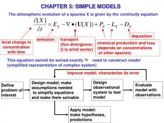
CHAPTER 3: SIMPLE MODELS. The atmospheric evolution of a species X is given by the continuity equation. deposition. emission. transport (flux divergence; U is wind vector). local change in concentration with time. chemical production and loss (depends on concentrations

CHAPTER 3: SIMPLE MODELS
E N D
Presentation Transcript
CHAPTER 3: SIMPLE MODELS The atmospheric evolution of a species X is given by the continuity equation deposition emission transport (flux divergence; U is wind vector) local change in concentration with time chemical production and loss (depends on concentrations of other species) This equation cannot be solved exactly e need to construct model (simplified representation of complex system) Improve model, characterize its error Design observational system to test model Design model; make assumptions needed to simplify equations and make them solvable Evaluate model with observations Define problem of interest Apply model: make hypotheses, predictions
Atmospheric “box”; spatial distribution of X within box is not resolved ONE-BOX MODEL Chemical production Chemical loss Inflow Fin Outflow Fout X L P D E Deposition Emission Lifetimes add in parallel: Loss rate constants add in series:
NO2 emitted by combustion, has atmospheric lifetime ~ 1 day:strong gradients away from source regions Satellite observations of NO2 columns
CO emitted by combustion, has atmospheric lifetime ~ 2 months:mixing around latitude bands Satellite observations
CO2 emitted by combustion, has atmospheric lifetime ~ 100 years:global mixing Assimilated observations
GLOBAL BOX MODEL FOR CO2 (Pg C yr-1) IPCC [2001] IPCC [2001]
ATMOSPHERIC CO2 TREND OVER PAST 25 YEARS IPCC [2007] mmol mol-1 is the proper SI unit; ppm, ppmv are customary units
SPECIAL CASE: SPECIES WITH CONSTANT SOURCE, 1st ORDER SINK Steady state solution (dm/dt = 0) Initial condition m(0) Characteristic time t = 1/k for • reaching steady state • decay of initial condition If S, k are constant over t >> t, then dm/dt g0 and mg S/k: quasi steady state
TWO-BOX MODELdefines spatial gradient between two domains F12 m2 m1 F21 Mass balance equations: (similar equation for dm2/dt) If mass exchange between boxes is first-order: e system of two coupled ODEs (or algebraic equations if system is assumed to be at steady state)
LATITUDINAL GRADIENT OF CO2 , 2000-2012 Illustrates long time scale for interhemispheric exchange; use 2-box model to constrain CO2 sources/sinks in each hemisphere http://www.esrl.noaa.gov/gmd/ccgg/globalview/
EULERIAN RESEARCH MODELS SOLVE MASS BALANCE EQUATION IN 3-D ASSEMBLAGE OF GRIDBOXES The mass balance equation is then the finite-difference approximation of the continuity equation. Solve continuity equation for individual gridboxes • Models can presently afford ~ 106 gridboxes • In global models, this implies a horizontal resolution of 100-500 km in horizontal and ~ 1 km in vertical • Drawbacks: “numerical diffusion”, computational expense
IN EULERIAN APPROACH, DESCRIBING THE EVOLUTION OF A POLLUTION PLUME REQUIRES A LARGE NUMBER OF GRIDBOXES Fire plumes over southern California, 25 Oct. 2003 A Lagrangian “puff” model offers a much simpler alternative
PUFF MODEL: FOLLOW AIR PARCEL MOVING WITH WIND CX(x, t) In the moving puff, wind CX(xo, to) …no transport terms! (they’re implicit in the trajectory) Application to the chemical evolution of an isolated pollution plume: CX,b CX In pollution plume,
COLUMN MODEL FOR TRANSPORT ACROSS URBAN AIRSHED Temperature inversion (defines “mixing depth”) Emission E In column moving across city, CX x 0 L
LAGRANGIAN RESEARCH MODELS FOLLOW LARGE NUMBERS OF INDIVIDUAL “PUFFS” C(x, to+Dt) Individual puff trajectories over time Dt ADVANTAGES OVER EULERIAN MODELS: • Computational performance (focus puffs on region of interest) • No numerical diffusion DISADVANTAGES: • Can’t handle mixing between puffs a can’t handle nonlinear processes • Spatial coverage by puffs may be inadequate C(x, to) Concentration field at time t defined by n puffs
LAGRANGIAN RECEPTOR-ORIENTED MODELING Run Lagrangian model backward from receptor location, with points released at receptor location only backward in time • Efficient cost-effective quantification of source influence distribution on receptor (“footprint”)