Download
1 / 43
430 likes | 541 Views
This workshop focuses on identifying interesting patterns within geometric streams, analyzing data from various sources including IP packets, sensor data, and transaction logs. It introduces concepts such as adaptive spatial partitioning and the Q-Digest algorithm for data aggregation. Participants will explore methods for visualizing point stream shapes, determining areas of high density, and conducting efficient data profiling. The approach emphasizes balancing coverage and precision as well as dynamic adaption to data distributions, making it particularly relevant for practical applications in sensor networks and stream processing.

E N D
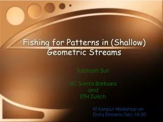
Fishing for Patterns in (Shallow) Geometric Streams Subhash Suri UC Santa Barbara and ETH Zurich IIT Kanpur Workshop on Data Streams Dec 18-20
Geometric Streams • A stream of points (dim 1, 2, 3, …) • Abstract view of multi-attribute data: • IP packets, database transactions, geographic sensor data, processor instruction stream etc. Worm DDoS IP Traffic (NetViewer) Sensor eScan Code profiling
Shape of a Point Stream • Form informs about the function • Identifying visually interesting patterns (“shape”) of point stream • Areas of high density (hot spots). • Large empty areas (cold spots). • Population estimates of geometric ranges • A geometric summary of the distribution of the stream. • Deliberately vague and ill-posed; some specifics later.
Outline • No attempt to survey • Adaptive Spatial Partitioning • Generic summary structure (Algorithmica ‘06) • Q-Digest: sensornet data aggregation (SenSys’04) • Range Adaptive Profiling for Programs (CGO ‘06) • Specialized geometric patterns and queries: • Range queries (SoCG ‘04) • Hierarchical Heavy-hitters (PODS ‘05) • Shape of the stream: ClusterHulls (Alenex‘06) • Conclusions
Adaptive Spatial Partitioning • A subdivision of space into square cells. • Each cell maintains O(1) size info, essentially count of points in it. • Tension between coverage and precision: • Large cells cover a lot, but with poor precision • Small cells have good precision, but poor coverage • Dynamically adapt the subdivision to the distribution of points in the stream. • Adaptive zoom: more precision (cells) where the action is, and fewer elsewhere. • [HSST], ISAAC ‘04, Algorithmica ‘06
ASP Structure L • Data structure size is function of accuracy parameter ε • Initially, a single box (LxL), and its counter. • When the count of a box b > εn • Freeze b’s counter • Split b into 4 sub-boxes • Introduce a new counter for each sub-box • This hierarchically defined structure of boxes (a streaming quad tree) is our ASP.
Refine operation Adaptivity: Refine and Unrefine • The structure must adapt to the changing distribution of points: • New regions become heavy • Previously heavy regions may become light/cold. • Refine operation puts new counters where the action is increasing: • Stream Processing: for each item x • Locate the smallest box v containing x, increment its count • Refine: If count of v > εN • Split v into 4 children sub-boxes, each with a new counter, initialized to 0. • Old counter of v frozen.
Unrefine Operation Unrefine operation • To conserve memory, boxes with low counts must be deleted. • A previously heavy box may become light because n, the size of the stream, has increased, and so its count is below εn. • Unrefine: if count of box v and its children < εn/2 • Delete the children boxes and • Add their counts to count of v • (v’s old counter revived) • Refinement occurs only at node of new insert; refinement can occur anywhere (non-locality). • A heap for fast unrefine ops.
L ASP-tree The Data Structure • ASP represented as a 4-ary tree
ASP-tree Analysis of ASP • (Space Bound): • For each node v, the count of v, its siblings, and parent > εn/2 • Total number of boxes at most O(1/ε) • (Per-point Processing Time): • Naïve will be O(lg L): tree height • With heap, centroid tree (amortized) time O(lg 1/ε) • (Count Bound): • Each point counted in exactly one box • Points contained in a box b are counted at b or one of its ancestors • Depth of the tree by the binary partitioning rule is O(log L) • Error in a leaf’s count is O(εn*log L). • Using memory = O(1/ε * log L), the count error bounded by εn.
Spatial Summary • A partition into O(1/ε * log L) boxes, with auto-adaptive zoom. • No undivided box has more than εn points: only leaf nodes can. • Gives a qualitative summary of the stream’s spatial distribution: a visual sense of hot and cold regions.
Two applications and two theorems • Data aggregation in sensor networks • Distributed version of ASP structure • Code profiling in processor streams • Hardware implementation of ASP • Theoretical bounds for range searching • Worst-case guarantees for rectangle range searching • Lower bounds on hierarchical heavy hitters • Space complexity
Geometric Summaries in Sensornets • Self-organizing networks of tiny, cheap sensors, • Integrated sensing, computing, radio communication, • Continuous, real-time monitoring of remote, hard to reach areas. • Limited power (battery), bandwidth, memory. • Communication typically the biggest drain on energy • Perform as much local processing as possible, and transmit smart summaries. • Similar to synopses: distributed data, rather than one-pass. • Active area: in-network aggregation, compressed sensing.
Base Station Distributed ASP • Q-Digest: an approximate histogram • Shrivastava, Buragohain, Agrawal, S. [SenSys ‘04] • ASP for 1-dim data signal (measurements of sensors): vibration data, acoustics, toxin levels, etc. • Going beyond min, max, or average, and approximating quantiles. • Sensors form an aggregation tree, rooted at base station. • Data flows from leaves to the base station, always reduced to size K summary. (user parameter). • The key point is that ASP is efficiently mergeable: • Given q-digests of children, a node can compute the merged q-digest. • Space/quality bounds of ASP carry over.
A simulation 8000 sensors,each generating a 2-byte integer (death valley elevation data) Error: (true - est) rank < 5% with 160 byte Q-Digest < 2% with 400 byte Q-Digest
Code Profiling Basic Blocks Code push %ebp mov %esp,%ebp sub $0x38,%esp and $0xfffffff0,%esp mov $0x0,%eax sub %eax,%esp sub $0x8,%esp push $0x28 push $0x8048468 call 80482b0 add push %ebp mov %esp,%ebp sub $0x38,%esp and $0xfffffff0,%esp mov $0x0,%eax sub %eax,%esp sub $0x8,%esp push $0x28 push $0x8048468 call 80482b0 add $0x10,%esppush %ebp mov %esp,%ebp sub $0x38,%esp and $0xfffffff0,%esp mov $0x0,%eax sub %eax,%esp sub $0x8,%esp push $0x28 push $0x8048468 call 80482b0 add $0x10,%espmov %esp,%ebp sub $0x38,%esp and $0xfffffff0,%esp mov $0x0,%eax sub %eax,%esp sub $0x8,%esp push $0x28 push $0x8048468 • Stream of program instructions • Profiling: Understand code behavior • Access patterns, cache behavior, load value distributions • Example: which program segments are hot, and how hot? • Challenges • Large item space: programs with 1M basic blocks • Profiling should take little space and add little overhead • ASP adaptation to profile high frequency code segments Frequent Rare
Range Adaptive Profiling [CGO ‘06] Hot range • Small fixed memory (counters) • Dynamically zoom onto high frequency code segments. • 1d adaptation of ASP with various “optimizations” to reduce memory and processing time. • Lot of constants squeezing • Batching of unrefinements • Branching factor choices • Design specs for specialized hardware for profiling (www.cs.ucsb.edu/~arch/rap) Cold range
Range Adaptive Profiling • Use RAP to estimate frequency of arbitrary ranges. • Count errors due to not splitting early enough • Regions undergoing hot/cold spells • Typical performance: 8K memory sufficient for 97% accuracy.
Yes, but…. That’s well and nice in practice, but how does it work in theory!
Range Searching in Streams • A stream of k-dimensional points. • Summary to approximate counts of geometric ranges. • VC dimension, -nets and -approximation. • “Nice” geometric ranges have small (bounded) VC dimension: e.g. rectangles, balls, half planes etc. • -approximation Theorem: For every range space (X, R) of fixed VC dim, there exists subset A of X of size O(lg s.t. • Iceberg error (n) unavoidable
-Approximations: challenges • Large summary size: (-2) • Would prefer O(1/ • -nets are small but can't estimate ranges • Deterministic construction a space hog. • The best streaming algorithm for -approximation requires working space O( (1/)d+1 lgO(d+1)n ) [BCEG ‘04]
Some Theorems [STZ, SoCG ‘04] • Deterministic Multipass: With d passes over data, can build a deterministic data structure for rectangular queries of size O(1/ lg2d-2 (1/. • Randomized Single pass: A data structure for rectangular range queries in 2d with error at most n, with prob > 1 - o(1), of size O(lgn The data structure size is only slightly sub-quadratic for d > 2:
B A C C Another Theorem • An implicit desire in ASP is to spot “pockets” of high population. • Think of such a spatially correlated set as a “spatial heavy hitter”: many different formal definitions possible. • An important concept is hierarchical heavy hitter (HHH). • Popularized by Estan-Varghese, Graham-Muthukrishnan • Non-redundant heavy hitters • Ranges often form a natural hierarchy (IP addresses, time, space, etc) • Stream of points and a (hierarchical) set of boxes. • Report boxes whose “discounted” frequency is above threshold. Discounted Frequency
C B A C B A Space Complexity of HHH [HSST, PODS ‘05] • Elegant applications to IP network monitoring, and clever algorithms by EV and CKMS • Unlike flat heavy hitters, however, 2-sided approximation guarantees seem difficult to achieve: • Every HHH (with discounted freq > n) should be caught • Every box reported must have discounted frequency > cn • HHH Space Theorem:Any -HHH algorithm in d dim with fixed accuracy factor c requires Ω(1/d+1) memory. Information loss in aggregation
Shape of a Point Stream Caution: entering highly speculative zone!!!
Shape of a Point Stream[HSS, Alenex ‘06] • What is a natural summary to describe the geometric shape of a streaming point set? • A simple first approximation is the convex hull, which preserves basic extremal properties: • Diameter, width, separation, containment, dist etc. • Efficient streaming Hulls [AHV, CM, Chan, FKZ, HS]. • Max error O(Diam/r2) for summary size r
Shape of a Point Stream • Convex hull is a crude summary when the point stream has a richer structure, especially in the interior. • Consider the simple example of L-shaped set. • A powerful technique for shape extraction is -hulls • area left after subtracting all 1/ radius empty disks • Unfortunately, -hulls can have linear size and we don’t know how to build a streaming approximation.
Cluster Hulls (ALENEX ‘06) • Generalizes the streaming convex hull algorithm to represent the shape as a collection of hulls. • Mimics -hull by using minimum area coverage as metric. • It is not clustering: • Objective is to approximate well the boundary shape of components • 2 dimensions only • Problems with noise • But could be coupled with clustering.
Algorithm: ClusterHulls • k convex hulls, H = {h1, h2,… hk} • A cost function w(h) = area(h) + μ(perimeter(h))2 • Minimize w(H) = Σw(hi) • For each point p in sequence • If p inside an hi, assign p to hi without modifying hi else create a new hull containing only p; add it to H • If |H| > k Choose a pair hi, hj to merge into a single hull, s.t. the increase to w(H) is minimized. • Revise the assignment of adaptive sampling directions to hulls in H to minimize the overall error.
Choosing the cost function • Area only: merges pairs of points from different clusters and intersecting hulls. • Perimeter only: favors merging of large hulls to reduce cost. • The combined area+perimeter works well at both extremes.
Some Pictures Input: West Nile Virus Data m = 256 m = 512 ClusterHulls
Why not Plain Clustering ClusterHulls k-median; k=5 CURE; k=5 m = 45 k-median; k=45 CURE; k=45
Extreme Examples • Early choices can be fatal. • Recover by discarding sparse CHs. • Process points in rounds whose length doubles each time. • Discard hulls h whose count(h) or density(h) = count(h)/area(h) is small. • On these extreme examples, most clustering algs fail Input ClusterHulls Period-doubling Cleanup
Conclusions, Open Problems • Is ClusterHull a good idea? • Too early to tell. The problem seems interesting. • Open theoretical questions: • Complexity of covering a set of points with convex polygons: at most k vertices, minimize the area. • Covering by rectangles (arbitrarily oriented). • Streaming versions? • Other notions of stream shape. • Space-efficient streaming range searching.
The Lower Bound in 1-D • r intervals of length 2 each (call them literals) • Union of the r intervals is B. • Each interval split into two unit length sub-intervals. • If stream points fall in the left (resp. right) subinterval, we say the literal has orientation 0 (resp. 1). B 2r Literal 0 1
The Construction • Stream arrives in 2 phases. • In 1st phase: Put 3N/r points in each interval, either in left or right half. • In 2nd phase: Adversary chooses either left or right half for each sub-interval and puts N points. Call these intervals sticks. • Heavy hitters: • Each stick is a -HHH • Discounted frequency of B (the union interval) depends on literals whose orientations in 1st and 2nd phase differ • Algorithms must keep track of (r) orientations after 1st phase B
The Lower Bound • Suppose an algorithm A uses < 0.01r bits of space. • After phase 1, orientations of the r literals encoded in 0.01r bits. • There are 2r distinct orientation • Two orientations that differ in at least r/3 literals map to the same (0.01r)-bit code ==> indistinguishable to A. • If orientations in 1st and 2nd phase are same, frequency of B = 0, not a HHH. • If r/3 literals differ, frequency of B = r/3 * 3N/r = N, so B is a -HHH • A misclassifies B in one sequence. B
Completing the Lower Bound 2r • Make r independent copies of the construction • Use only one of them to complete the construction in the 2nd phase • Need (r2) bits to track all orientations • For r = 1/4, this gives (j-2) lower bound B r
Multi-dimensional lower bound • The 1-D lower bound is information-theoretic; applies to all algorithms. • For higher dimensions, need a more restrictive model of algorithms. • Box Counter Model. • Algorithm with memory m has m counters • These counters maintain frequency of boxes • All deterministic heavy hitter algorithms fit this model • In the box counter model, finding -HHH in d-dim with any fixed approximation requires (d+1) memory
0 1 Literal Diagonal Uniform Stick 2r 2D (Multi-Dim) Construction • A box B and a set of descendants. • B has side length 2r. • 1st phase • 2x2 (literal) boxes in upper left quadrant (orientation 0 or 1) • 2nd phase • Diagonal: boxes in upper left quadrant; all orientation 0 • Sticks: 1xr (or rx1) boxes • Uniform: lower right quadrant
FullyCovered Half Covered Multi-dimensional lower bound • Intuition: • Each stick combines with a diagonal box to form a skinny -HHH box • Diagonal boxes pair-up to form -HHH • Skinny boxes form a checker-board pattern in upper left quadrant • Each literal is either fully covered or half covered • As in 1-D, adversary picks sticks • Discounted frequency of B has • Half covered literals and • Points in the Uniform quadrant Diagonal Uniform Stick 2r
The Lower Bound • The algorithm must remember the W(r2) literal orientations. • Otherwise, it cannot distinguish between two sequences, where discounted frequency of B is m or 3m/2, resp. (for m = 20/29 N). • Like before, by making r copies of the construction, we get the lower bound of W(r3). • The basic construction generalized to d dimensions. • Adjusting the hierarchy to get lower bound for any arbitrary approximation