Download
1 / 30
300 likes | 500 Views
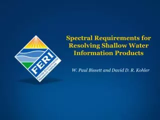
Spectral Requirements for Resolving Shallow Water Information Products. W. Paul Bissett and David D. R. Kohler. Optically-Deep. Optically-Shallow. Whitecaps. Micro-bubbles. Shallow Ocean Floor. Suspended Sediments. Phytoplankton. Benthic Plants. 1/Kd. CDOM-Rich Water.

E N D
Spectral Requirements for Resolving Shallow Water Information Products W. Paul Bissett and David D. R. Kohler
Optically-Deep Optically-Shallow Whitecaps Micro-bubbles Shallow Ocean Floor Suspended Sediments Phytoplankton Benthic Plants 1/Kd CDOM-Rich Water Coastal Ocean Imaging Spectroscopy
Spectral Resolution Depth = 6.5 m IOP = Case 1 Bottom = soft coral Depth = 13 m IOP = Pure H20 Bottom = sponge
Why (Hyper) Spectral? • Discriminate analysis suggests 10-12 independent vectors of information in hyperspectral data stream. • But which bands are a priori the rights one to measure? • Additional bands give greater degrees of freedom with which to attempt more complicated inversion algorithms to retrieve depth-dependent IOPs, which include products such as bathymetry, in situ IOPs, bottom classification.
1.9 x 10⁶ Total Points 39% of the LUT results are +/- 10% 73% of the LUT results are +/- 25% A normal distribution is plotted for reference. The LUT results have less error than would be expected for a normally distributed population.
NOAA/Florida Marine Research InstituteBenthic Assessment of the Florida Keys
Sand Seagrass Coral Hardbottom Comparison of LUT and NOAA Bottom Types FERI LUT 2002 NOAA 1992 • 16 m resolution • Unknown pixels removed from both data sets.
Evidence of Algal Overgrowth in the Florida Keys Typical algal overgrowth on coral rubble in Florida. Photo courtesy of U.S. Department of the Interior, U.S. Geological Survey, Center for Coastal Geology Caulerpa brachypus is a nonnative macroalgae that has invaded Florida's coral reefs. Photo courtesy of Harbor Branch Oceanographic Institution, Inc.
Simulating Impacts of Sensor Design • Created 216K different hyperspectral Rrs(λ) spectra with various water depths, IOPs, and bottom reflectance spectra. • These spectra were used to create reduced resolution spectra of 5, 15, 25, and 35 nm continuous spectra to test impact of sensor spectral resolution and radiometric discretization.
Spectral Resolution in Shallow Water(OC4) 9,754 Hydrolight runs with various depths (0.1 – 20 meters), IOPs (25 with chl = 0.0. to 0.2), bottom reflectances (60 different spectra). Max[Rrs(443), Rrs(490), Rrs(510)] /Rrs(555) = 1.0 ± 0.005 OC4 Chlorophyll a = 2.32 mg/m3
Radiometric Discretization Depth = 25 m IOP = Case 1 / chl of 2 mg/m3 Bottom = clean sand Dynamic Range was set so that the sensor would not saturate over dry sand. However, the Rrs does not include atmosphere. Inclusion of the atmosphere would dramatically worsen this discretization error, since most of the signal is from the atmosphere, and the bit resolution of the dark signals would thereby be lessened.
Requirements Analysis • 216k simulated shallow water reflectance spectra • Resampled each to represent different combinations of sensor bit levels (8, 10, 12, and 14) and band widths (5, 15, 25, and 30) • Found the absolute spectral difference from the original and resampled spectra to determine the amount of information lost due to the configuration • 1) Σ {absolute[ Rrs(λ) – Rrs_resample(λ)]} • 2) Average (absolute{ [ Rrs(λ) – Rrs_resample(λ)] / Rrs(λ) } )
Histogram of Average Relative Error (Focus on Discretization)
Contours of 3-D Avg Rel Err Surface (Viewed from Top) Percentage of counts per Bit Level that fell beyond 50% relative error: 14 bit – 0.00% 12 bit – 0.02% 10 bit – 10.92% 8 bit – 41.92%
Contours of 3-D Avg Rel Err Surface (Viewed from Top) Percentage of counts per Bit Level that fell beyond 50% relative error: 14 bit – 0.01% 12 bit – 0.02% 10 bit – 6.51% 8 bit – 34.97%
Contours of 3-D Avg Rel Err Surface (Viewed from Top) Percentage of counts per Bit Level that fell beyond 50% relative error: 14 bit – 0.45% 12 bit – 0.56% 10 bit – 7.82% 8 bit – 36.55%
Contours of 3-D Avg Rel Err Surface (Viewed from Top) Percentage of counts per Bit Level that fell beyond 50% relative error: 14 bit – 0.96% 12 bit – 1.89% 10 bit – 8.23% 8 bit – 35.28%
Contours of 3-D Avg Rel Err Surface (Viewed from Top) Percentage of counts per width that fell beyond 50% relative error: 35 nm – 0.96% 25 nm– 0.45% 15 nm– 0.01% 5 nm– 0.00%
Contours of 3-D Avg Rel Err Surface (Viewed from Top) Percentage of counts per width that fell beyond 50% relative error: 35 nm – 1.89% 25 nm– 0.56% 15 nm– 0.02% 5 nm– 0.02%
Contours of 3-D Avg Rel Err Surface (Viewed from Top) Percentage of counts per width that fell beyond 50% relative error: 35 nm – 8.23% 25 nm– 7.82% 15 nm– 6.51% 5 nm– 10.92%
Contours of 3-D Avg Rel Err Surface (Viewed from Top) Percentage of counts per width that fell beyond 50% relative error: 35 nm – 35.28% 25 nm– 36.55% 15 nm– 34.97% 5 nm– 41.92%
Summary • Imaging spectroscopy can address the requirement to simultaneous solve for bathymetry, IOPs, and bottom reflectance in the shallow water environment. This will allow for the production of robust image products, including water clarity, extreme phytoplankton concentrations (red and brown tides), resuspended sediments, river discharges. • This analysis suggests there may be little difference between 12 and 14 bits discretization, and 5 and 10 nm band width. • However, this analysis does not include TOA reflectance, which will reduce the bit resolution of the Rrs. • It also does not include noise, which will impact the simulated results.
Summary • The real issue are how the impacts of the requirements affect image products. These products require new algorithms, which to date have not been completely developed and tested (cart and horse problem). • One of the issues not addressed in this study is that average percentage errors are not the same as reduce spectral information. • The requirements for resolution, calibration, and SNR should be driven by product generation. • Real high spatial and spectral data sets exist, with future collections planned, that may be used to develop these products.
Monterey Bay CICORE Central California 2002 Total Kelp : 3.93 sq km Total Kelp : 2.99 sq km Big Sur Total Kelp : 1.11 sq km Total Kelp : 5.73 sq km Total Kelp : 0.55 sq km Total Kelp : 0.76 sq km Morro Bay San Luis Bay