Understanding Normal Distribution and Related Theorems for Statistics
150 likes | 250 Views
Learn about normal distribution, standard deviation, and important theorems in statistics. Solve exercises to understand probabilities with the standard normal distribution.

Understanding Normal Distribution and Related Theorems for Statistics
E N D
Presentation Transcript
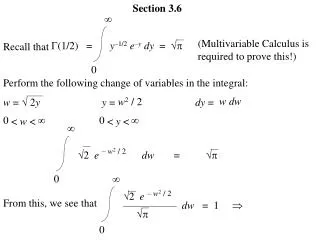
Section 3.6 Recall that (Multivariable Calculus is required to prove this!) (1/2) = y–1/2e–y dy = 0 Perform the following change of variables in the integral: w = 2yy = dy = < w < < y < w dw w2 / 2 0 0 – w2 / 2 2 e dw = 0 – w2 / 2 2 e ————— dw = 1 From this, we see that 0
– w2 / 2 – w2 / 2 2 e ————— dw = 2 e ——— dw = 1 2 – – Let –< a < and 0 < b < , and perform the following change of variables in the integral: x = a + bww = dw = < x < < w < We shall come back to this derivation later. Right now skip to the following: A random variable having this p.d.f. is said to have a normal distribution with mean and variance 2, that is, a N(,2) distribution. A random variable Z having a N(0,1) distribution, called a standard normal distribution, has p.d.f. – z2 / 2 e f(z) = ——— for –< z < 2
We let (z) = P(Z z), the distribution function of Z. Since f(z) is a symmetric function, it is easy to see that (– z) = 1 – (z). Tables Va and Vb in Appendix B of the text display a graph of f(z) and values of (z) and (– z). Important Theorems in the Text: If X is N(,2), then Z = (X– ) / is N(0,1). Theorem 3.6-1 If X is N(,2), then V = [(X – ) / ]2 is 2(1). Theorem 3.6-2 We shall discuss these theorems later. Right now go to Class Exercise #1:
1. The random variable Z is N(0, 1). Find each of the following: P(Z < 1.25) = (1.25) = 0.8944 P(Z > 0.75) = 1 – (0.75) = 0.2266 P(Z < – 1.25) = (– 1.25) = 1 – (1.25) = 0.1056 P(Z > – 0.75) = 1 – (– 0.75) = 1 – (1 – (0.75)) = (0.75) = 0.7734 P(– 1 < Z < 2) = (2)– (– 1) = (2)– (1 – (1)) = 0.8185 P(– 2 < Z < – 1) = (– 1)– (– 2) = (1 – (1))– (1 – (2)) = 0.1359 P(Z < 6) = (6) = practically 1
a constant c such that P(Z < c) = 0.591 P(Z < c) = 0.591 (c) = 0.591 c = 0.23 a constant c such that P(Z < c) = 0.123 P(Z < c) = 0.123 (c) = 0.123 1 – (– c) = 0.123 (– c) = 0.877 – c = 1.16 c = –1.16 a constant c such that P(Z > c) = 0.25 P(Z > c) = 0.25 1 – (c) = 0.25 c 0.67 a constant c such that P(Z > c) = 0.90 P(Z > c) = 0.90 1 – (c) = 0.90 (– c) = 0.90 – c = 1.28 c = –1.28
1.-continued z0.10 P(Z > z) = 1 – (z) = z0.10 = 1.282 z0.90 P(Z > z) = 1 – (z) = (–z) = 1 – (–z) = 1 – P(Z > –z) = 1 – z1– = –z z0.90 = – z0.10 = –1.282 a constant c such that P(|Z| < c) = 0.99 P(– c < Z < c) = 0.99 P(Z < c) – P(Z < – c) = 0.99 (c) –(– c) = 0.99 (c) –(1 – (c)) = 0.99 (c) = 0.995 c = z0.005 = 2.576
– w2 / 2 – w2 / 2 2 e ————— dw = 2 e ——— dw = 1 2 – – Let –< a < and 0 < b < , and perform the following change of variables in the integral: x = a + bww = dw = < x < < w < (x – a) / b (1/b) dx – – (x – a)2 – ——— 2b2 The function of x being integrated can be the p.d.f. for a random variable X which has all real numbers as its space. e ———— dx = 1 b2 –
The moment generating function of X is M(t) = E(etX) = (x – a)2 – ——— 2b2 (x – a)2 –2b2tx – —————— 2b2 etx e ———— dx = b2 e ———— dx = b2 – – Let us consider the exponent (x – a)2 –2b2tx – —————— 2b2 exp{ } —————————— dx b2 (x – a)2 –2b2tx – —————— . 2b2 – (x – a)2 –2b2tx – —————— = 2b2 x2 – 2ax + a2 –2b2tx – ————————— = 2b2 x2 – 2(a + b2t)x + (a + b2t)2 – 2ab2t – b4t2 – ————————————————— = 2b2
[x–(a + b2t)]2 – 2ab2t – b4t2 – ———————————— . Therefore, M(t) = 2b2 (x – a)2 –2b2tx – —————— 2b2 exp{ } —————————— dx = b2 – [x –(a+b2t)]2 – —————— 2b2 b2t2 exp{at + ——} 2 b2t2 at + —— 2 exp{ } —————————— dx = b2 e – b2t2 at + —— 2 M(t) = e for –< t < b2t2 at + —— 2 M(t) = (a + b2t) e b2t2 at + —— 2 b2t2 at + —— 2 M(t) = (a + b2t)2e + b2 e
E(X) = M(0) = a E(X2) = M(0) = a2 + b2 Var(X) = a2 + b2– a2= b2 Since X has mean = and variance 2 = , we can write the p.d.f of X as a b2 (x –)2 – ——— 22 e f(x) = ———— for –< x < 2 A random variable having this p.d.f. is said to have a normal distribution with mean and variance 2, that is, a N(,2) distribution. A random variable Z having a N(0,1) distribution, called a standard normal distribution, has p.d.f. – z2 / 2 e f(z) = ——— for –< z < 2
We let (z) = P(Z z), the distribution function of Z. Since f(z) is a symmetric function, it is easy to see that (– z) = 1 – (z). Tables Va and Vb in Appendix B of the text display a graph of f(z) and values of (z) and (– z). Important Theorems in the Text: If X is N(,2), then Z = (X– ) / is N(0,1). Theorem 3.6-1 If X is N(,2), then V = [(X – ) / ]2 is 2(1). Theorem 3.6-2
2. The random variable X is N(10, 9). Use Theorem 3.6-1 to find each of the following: 6 – 10 X– 10 12 – 10 P( ——— < ——— < ———— ) = 3 3 3 P(6 < X < 12) = P(– 1.33 < Z < 0.67) = (0.67)– (– 1.33) = (0.67)– (1 – (1.33)) = 0.7486 – (1 – 0.9082) = 0.6568 X– 10 25 – 10 P( ——— > ———— ) = 3 3 P(X > 25) = P(Z > 5) = 1 – (5) = practically 0
2.-continued a constant c such that P(|X – 10| < c) = 0.95 X– 10 c P( ——— < — ) = 0.95 3 3 P(|X – 10| < c) = 0.95 P(|Z| < c/3) = 0.95 (c/3) –(– c/3) = 0.95 (c/3) –(1 – (c/3)) = 0.95 (c/3) = 0.975 c/3 = z0.025 = 1.960 c = 5.880
3. The random variable X is N(–7, 100). Find each of the following: X+ 7 0 + 7 P( ——— > —— ) = 10 10 P(X > 0) = P(Z > 0.7) = 1 – (0.7) = 0.2420 a constant c such that P(X > c) = 0.98 X+ 7 c +7 P( —— > —— ) = 0.98 10 10 P(X > c) = 0.98 P(Z > (c+7) / 10) = 0.98 1 – ((c+7) /10) = 0.98 ((c+7) /10) = 0.02 (c+7) /10 = z0.98 = –z0.02 = – 2.054 c = – 27.54
3.-continued X2+ 14X + 49 —————— 100 the distribution for the random variable Q = X2+ 14X + 49 —————— = 100 From Theorem 3.6-2, we know that Q = 2 X + 7 —— 10 must have a distribution. 2(1)