Download
1 / 11
120 likes | 169 Views
Explore exponential smoothing examples for Port of Baltimore to evaluate accuracy of constant and for Midwestern Manufacturing predicting demand trends using regression model.

E N D
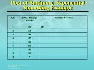
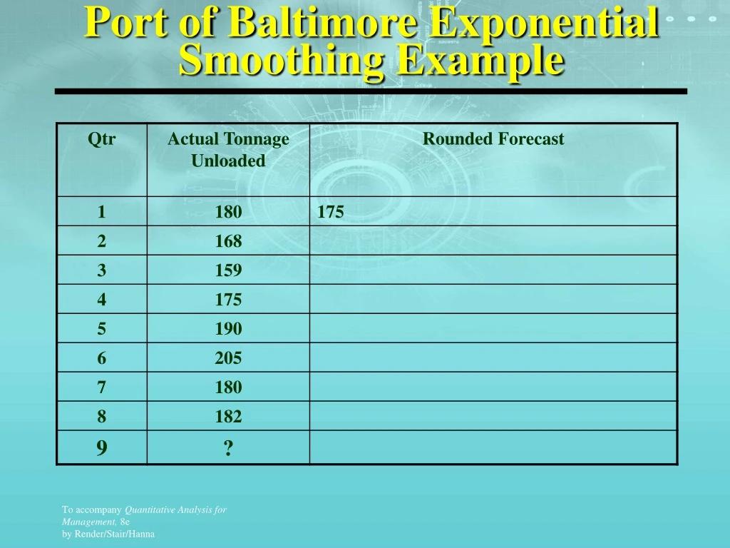
Port of Baltimore Exponential Smoothing Example • To evaluate the accuracy of each smoothing constant, we can compute the absolute deviations and MADs.
Port of Baltimore Exponential Smoothing Example • Based on this analysis, a smoothing constant of =0.10 is preferred to =0.50 because its MAD is smaller.
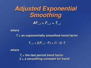
Trend Projections • A trend line is simply a linear regression equation in which the independent variable (X) is the time period. The form is a = - b
Example/Midwestern Manufacturing Company • Let us consider the case of Midwestern Manufacturing Company. That firm's demand for electrical generators over the period 1996-2002 is shown in the table below:
Example/Midwestern Manufacturing Company • A trend line to predict demand (Y) based on the period can be developed using a regression model. • We let 1996 be time period 1 (X = 1) then 1997 is time period 2 (X = 2), and so forth.
Example/Midwestern Manufacturing Company a = 98.86- 10.54(4)=56.7 • Hence, the least squares trend equation is Y= 56.70 + 10.54 X. • To project demand in 2003, we first denote the year 2003 in our new coding system as X = 8 • (sales in 2003) = 56.7 + 10.54 (8) = 141 generators • (sales in 2004) = 56.7 + 10.54 (9) = 152 generators