Fitting Regression Models

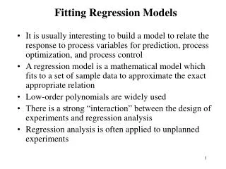
1. Fitting Regression Models • It is usually interesting to build a model to relate the response to process variables for prediction, process optimization, and process control • A regression model is a mathematical model which fits to a set of sample data to approximate the exact appropriate relation • Low-order polynomials are widely used • There is a strong “interaction” between the design of experiments and regression analysis • Regression analysis is often applied to unplanned experiments

2. Linear Regression Models • In general, the response variable y may be related to k regressor variables by a multiple linear (first order) regression model y = bo + b1x1 + b2x2 +  + bkxk + e • Models of more complex forms can be analyzed similarly. E.g., y = bo + b1x1 + b2x2 + b12x1x2 + e => y = bo + b1x1 + b2x2 + b3x3 + e • Any regression model that is linear in the parameters (b values) is a linear regression model, regardless of the shape of the response surface • The variables have to be quantitative

3. Model Fitting – Estimating Parameters • The method of least squares is typically used • Assuming that the error term e are uncorrelated random variables • The data can be expressed as • The model equation is yi = bo + b1xi1 + b2xi2 +  + bkxik + ei • Least square method chooses the b´s so that the sum of the squares of the errors ei is minimized

4. Model Fitting – Estimating Parameters • The least squares function is • The least squares estimators ( ) must satisfy • and • or

5. Model Fitting – Estimating Parameters • Or in the matrix notation • y = Xb + e • The least squares estimators of b are • The fitted model and residuals are • Example 10-1: • Response: viscosity of a polymer (y) • Variables: reaction temperature (x1), catalyst feed rate (x2) • The model • y = bo + b1x1 + b2x2 + e

9. Fitting Regression Models in Designed Experiments • Example 10-2: regression analysis of a 23 factorial design • Response: yield of a process • Variables: temperature, pressure, and concentration • Single replicate with 4 center points

10. Fitting Regression Models in Designed Experiments • A main effects only model • y = bo + b1x1 + b2x2 + b3x3 + e

11. Fitting Regression Models in Designed Experiments • The regression coefficients are exactly one-half of the effect estimates in a 2k design • Because the factorial designs are orthogonal designs, the off-diagonal elements in X´X are zero, or X´X is diagonal • Regression method is useful when the experiment (or data) is not perfect • Regression analysis of data with missing observations. Example 10-3: assuming run 8 of the observations in Example 10-2 was missing. Fit the main effect model using the remaining observations • y = bo + b1x1 + b2x2 + b3x3 + e

12. Example 10-3 Original model

13. Fitting Regression Models in Designed Experiments • Regression analysis of experiments with inaccurate factor levels • Example 10-4: assuming the process variables are not at their exact assumed values in Example 10-2. Fit the main effect model y = bo + b1x1 + b2x2 + b3x3 + e

14. Example 10-4 Original model

15. Fitting Regression Models in Designed Experiments • Regression analysis can be used to de-alias interactions in a fractional factorial using fewer than a full fold-over fraction in a resolution III design • Example 10-5: consider Example 8-1, assume effects A, B, C, D, and AB+CD were large – de-alias AB+CD using fewer than 8 additional runs. Consider the model • y = bo + b1x1 + b2x2 + b3x3 + b4x4 + b12x1x2 + b34x3x4 + e

16. The X matrix for the model is • Adding one run from the alternate fraction to the original 8 runs, the X matrix becomes

17. Hypothesis Testing in Multiple Regression • Measuring the usefulness of the model • Test for significance of regression – determine if there is a linear relationship between the response y and a subset of the regressor variables x1, x2, , xk. • Testing hypothesis • Ho: b1 = b2 = = bk = 0 • H1: bj 0 for at least one j • Analysis of variance • SST = SSR + SSE

18. Hypothesis Testing in Multiple Regression • If Fo exceeds Fa,k,n-k-1, the null hypothesis is rejected

20. Hypothesis Testing in Multiple Regression • Testing individual and group of coefficients – determine if one or a group of regressor variables should be included in the model • Testing hypothesis (for an individual regression coefficient) • Ho: bj = 0 • H1: bj 0 • if Ho is not rejected, then xj can be deleted from the model. • Ho is rejected if |to| > ta/2,n-k-1

21. The contribution of a particular variable, or a group of variables can be quantified using sums of squares • Confidence intervals on individual regression coefficients • Example 10-7

22. Prediction of new response observations • The future observation yo at a point (xo1, xo2, ,xok) with x’o =[1, xo1, xo2, ,xok] • Regression model diagnostics • Testing for lack of fit • Sections 10-7, 8