Regression Models
Regression Models. Professor William Greene Stern School of Business IOMS Department Department of Economics. Regression and Forecasting Models. Part 1 – Simple Linear Model. Theory. Demand Theory: Q = f(Price) “The Law of Demand” Demand curves slope downward

Regression Models
E N D
Presentation Transcript
Regression Models Professor William Greene Stern School of Business IOMS Department Department of Economics
Regression and Forecasting Models Part 1 – Simple Linear Model
Theory • Demand Theory: Q = f(Price) • “The Law of Demand” Demand curves slope downward • What does “ceteris paribus” mean here?
Data on the U.S. Gasoline Market Quantity = G = Expenditure / Price
Is There a Theory for This? Scatter plot of box office revenues vs. number of “Can’t Wait To See It” votes on Fandango for 62 movies.
Average Box Office by Internet Buzz Index= Average Box Office for Buzz in Interval
Deterministic Relationship: Not a Theory Expected High Temperatures, August 11-20, 2013, ZIP 10012, NY
Probabilistic RelationshipWhat Explains the Noise? Fuel Bill = Function of Rooms + Random Variation
The Regression Model y = 0 + 1x + y = dependent variable x = independent variable The ‘regression’ is the deterministic part, 0 + 1x The ‘disturbance’ (noise) is . The regression model is E[y|x] = 0 + 1x
y E[y|x] = 0 + 1x 1 = slope 0 = y intercept x Linear Regression Model
The Model • Constructed to provide a framework for interpreting the observed data • What is the meaning of the observed relationship (assuming there is one) • How it’s used • Prediction: What reason is there to assume that we can use sample observations to predict outcomes? • Testing relationships
The slope is the interesting quantity.Each additional year of education is associated with an increase of 3.611 in disability adjusted life expectancy.
A Cost Model Electricity.mpj Total cost in $Million Output in Million KWH N = 123 American electric utilities Model: Cost = 0 + 1KWH + ε
Interpreting the Model • Cost = 2.44 + 0.00529 Output + e • Cost is $Million, Output is Million KWH. • Fixed Cost = Cost when output = 0 Fixed Cost = $2.44Million • Marginal cost = Change in cost/change in output= .00529 * $Million/Million KWH= .00529 $/KWH = 0.529 cents/KWH.
Covariation and Causality Does more education make you live longer (on average)?
Causality? Estimated Income = -451 + 50.2 Height Height (inches) and Income ($/mo.) in first post-MBA Job (men). WSJ, 12/30/86. Ht. Inc. Ht. Inc. Ht. Inc. 70 2990 68 2910 75 3150 67 2870 66 2840 68 2860 69 2950 71 3180 69 2930 70 3140 68 3020 76 3210 65 2790 73 3220 71 3180 73 3230 73 3370 66 2670 64 2880 70 3180 69 3050 70 3140 71 3340 65 2750 69 3000 69 2970 67 2960 73 3170 73 3240 70 3050
How to compute the y intercept, b0, and the slope, b1, in y = b0 + b1x. b1 b0
Fitting a Line to a Set of Points Yi Gauss’s methodof least squares. Residuals Predictionsb0+ b1xi Choose b0and b1tominimize the sum of squared residuals Xi
b1= 72.718 b0=-14.36
Least squares minimizes the sum of squared deviations from the line.
Summary • Theory vs. practice • Linear Relationship • Deterministic • Random, stochastic, ‘probabilistic’ • Mean is a function of x • Regression Relationship • Causality vs. correlation • Least squares


