Download
1 / 26
320 likes | 560 Views
Stabilization of Galerkin Reduced Order Models (ROMs) for LTI Systems Using Controllers. Irina Kalashnikova 1 , Bart G. van Bloemen Waanders 1 , Srinivasan Arunajatesan 2 , Matthew F. Barone 2

E N D
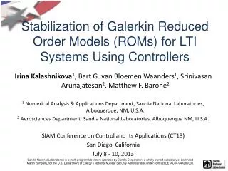
Stabilization of Galerkin Reduced Order Models (ROMs) for LTI Systems Using Controllers Irina Kalashnikova1, Bart G. van Bloemen Waanders1, Srinivasan Arunajatesan2, Matthew F. Barone2 1 Numerical Analysis & Applications Department, Sandia National Laboratories, Albuquerque, NM, U.S.A. 2Aerosciences Department, Sandia National Laboratories, Albuquerque NM, U.S.A. SIAM Conference on Control and Its Applications (CT13) San Diego, California July 8 - 10, 2013
Why Develop a Reduced Order Model (ROM)? High-fidelity modeling is often too expensive for use in a design or analysis setting! A Reduced Order Model (ROM) is a surrogate model that aims to capture the essential dynamics of a full numerical model but with far fewer dofs. • Example Applications of ROMs: • Aeroelastic flutter analysis. • System modeling for active flow control. • Design/analysis of microelectromechanical devices and systems (MEMS) under electric actuation. 1/21
Proper Orthogonal Decomposition (POD)/Galerkin Method to Model Reduction 2/21
Step 1: Proper Orthogonal Decomposition (POD) Algorithm (a.k.a., “Method of Snapshots”) Collect snapshots of a solution vector . Place these snapshots into the columns of a matrix defined by , …, 2. Select an inner product to build the reduced basis in, e.g., the inner product. 3. Compute the SVD of the matrix 4. A reduced POD basis of size is given by ) 5. Orthonormalize and return the reduced basis. # of dofs in high-fidelity simulation # of snapshots # of dofs in ROM (, ) Truncated POD basis describes more energy (on average) of the snapshot set than any other linear basis of the same dimension . 3/21
Step 2: Galerkin Projection LTI Full Order Model (FOM) dofs Approximate solution as a linear combination of the POD modes obtained in Step 1: 2. Project FOM system onto the modes in some inner product, e.g., the inner product to obtain… ROM solution LTI Reduced Order Model (ROM) dofs 4/21
Stability Issues of POD/Galerkin ROMs LTI Full Order Model (FOM) LTI Reduced Order Model (ROM) • ROM LTI system matrices given by: • , Problem: stable stable! • There is no a priori stability guarantee for POD/Galerkin ROMs. • Stability of a ROM is commonly evaluated a posteriori – RISKY! • ROM instability of POD/Galerkin ROMs is a real problem in some applications (e.g., compressible flow). 5/21
Stability Preserving Model Reduction Approaches: Literature Review Approaches for building stability-preserving POD/Galerkin ROMs found in the literature fall into two categories: • 1. ROMs which derive a prioria stability-preserving model reduction framework (usually specific to an equation set). • ROMs based on projection in special ‘energy-based’ (not ) inner products, e.g., Rowley et al. (2004), Barone & Kalashnikova et al. (2009), Serre et al. (2012). • 2. ROMs which stabilize an unstable ROM through an a posteriori post-processing stabilization step applied to the algebraic ROM system. • Petrov-Galerkin ROMs that solve an optimization problem for the test basis given a trial POD basis, e.g., Amsallem et al. (2012), Bond et al. (2008). • ROMs with increased numerical stability due to inclusion of ‘stabilizing’ terms (e.g., LES terms) in the ROM equations, e.g., Wang, Akhtar, Borggaard, Iliescu(2012) Potentially intrusive implemetation Inconsistencies between ROM and FOM physics 6/21
New ROM Stabilization Approach: ROM Stabilization via Pole Placement New ROM Stabilization Idea (falling under second category of ROM stabilization methods): Make ROM system matrix stable through pole (eigenvalue) placement LTI FOM: stable LTI ROM: unstable • Pick a control matrix . • Modify LTI ROM by adding to it the control : • Assume linear control of the form : • Compute the feedback matrix such that • has desired (stable) poles. • Open Questions: • How to pick ? • What eigenvalues should have? • Does solution to pole placement problem exist? • How does stabilization affect ROM accuracy? 7/21
Algorithm #1: ROM Stabilization via Pole Placement • Ensures the solution to the pole placement problem exists. Theorem (from Aströmet al. 2009): If the pair (AM,BC) is controllable, there exists a feedback such that the eigenvalues of can be arbitrarily assigned. • Algorithm #1 Outline • Given , use Kalman decomposition to isolate controllable and observable part of and , call them , . • Compute eigenvalues of . • Reassign unstable eigenvalues of , e.g., set • Compute such that has these eigenvalues using pole placement algorithms from control theory. • Set ). 8/21
Numerical Results: International Space Station (ISS) Benchmark Stabilized via Algorithm #1 Component 1r • FOM: structural model of component 1r (Russian service module) of the International Space Station (ISS). • matrices defining FOM downloaded from NICONET model reduction benchmark repository. • No inputs (unforced) 1 output; FOM is stable 9/21
Numerical Results: ISS Benchmark Stabilized via Algorithm #1 (continued) • POD/Galerkin ROM constructed using snapshots collected until time . • POD/Galerkin ROM has 4 unstable eigenvalues. • (stabilization matrix selected to be vector of all 1s). 10/21
Selecting ROM Eigenvalues (Poles) • If ROM is stable, ROM eigenvalues will lie on same manifold as FOM eigenvalues. • In fact, if and ROM is stable, , so eig()=eig(). • However: if ROM is unstable, ROM eigenvalues can be chaotic. Could try to place ROM poles to match FOM poles… …but this does not ensure accuracy of ROM! 11/21
Algorithm #2: ROM Stabilization Optimization Problem • Ensures stabilized ROM solution deviates minimally from FOM solution. Key Idea: An exact solution to the ROM LTI system can be derived using the matrix exponential. • Recall that the ROM LTI system is given by • The solution to the ROM LTI system is: 12/21
Algorithm #2: ROM Stabilization Optimization Problem (continued) ROM Stabilization Optimization Problem (Constrained Nonlinear Least Squares): • = unstable eigenvalues of original ROM matrix . • snapshot output at • ROM output at . • ROM stabilization optimization problem is small: • ROM stabilization optimization problem can be solved by standard optimization algorithms, e.g., interior point method. • We use fmincon function in MATLAB’s optimization toolbox. • We implement ROM stabilization optimization problem in characteristic variables where . 13/21
Algorithm #2 Is Equivalent to Specific Instance of Algorithm #1 (Pole Placement Problem) • Let be the new ROM matrix following stabilization by Algorithm #2: • , stabilized by Algorithm #2 Can show: Algorithm #2 is equivalent to Algorithm #1 (Pole Placement Problem) for a specific and . • One can show that where (WLOG, if 2 eigenvalues were stabilized): • Here: • denotes the original (unstable) eigenvalue of • denotes the new (stable) eigenvalue of computed by Algorithm #2. • denotes matrix of eigenvectors of . 14/21
Numerical Results: ISS Benchmark Stabilized via Algorithm #2 • POD/Galerkin ROM has 4 unstable eigenvalues: 2 real, 2 complex • Two options for ROM stabilization optimization problem: • Option 1:Solve for s.t. the constraint . • Option 2: Solve for , ,,s.t. the constraint • Initial guess for fmincon interior point method: . 15/21
Numerical Results: Electrostatically Actuated Beam Benchmark Stabilized via Algorithm #2 • FOM = 1D model of electrostatically actuated beam. • Application of model: microelectromechanical systems (MEMS) devices such as electromechanical radio frequency (RF) filters. • 1 input corresponding to periodic on/off switching, 1 output, initial condition . • Second order linear semi-discrete system of the form: • Matrices , , , , specifying the problem downloaded from the Oberwolfach model reduction repository. • 2nd order linear system re-written as 1st order LTI system for purpose of analysis/model reduction. • FOM is stable. 16/21
Numerical Results: Electrostatically Actuated Beam Benchmark Stabilized via Algorithm #2 (continued) • POD/Galerkin ROM constructed from snapshots up to time . • POD/Galerkin ROM has 4unstable eigenvalues (all real). • Two options for ROM stabilization optimization problem: • Option 1:Solve for s.t. the constraint . • Option 2: Solve for , ,,s.t. the constraint • Initial guess for fmincon interior point method: . 17/21
Numerical Results: Electrostatically Actuated Beam Benchmark Stabilized via Algorithm #2 (continued: stabilized poles) 18/21
Summary & Future Work • A new ROM stabilization approach that modifies a posteriori an unstable ROM LTI system by changing the system’s unstable eigenvalues is proposed. • It is demonstrated how an unstable ROM’s eigenvalues may be placed using ideas from control theory, i.e., pole placement assuming a linear control (Algorithm #1). • It is unclear how stabilization via Algorithm #1 will affect the accuracy of the ROM. • To address this, a constrained nonlinear least squares optimization problem for the ROM eigenvalues is formulated (Algorithm #2). • It is shown that Algorithm #2 is equivalent to Algorithm #1 for a specific linear control. • Performance of the proposed algorithms is evaluated on two benchmarks. • Ongoing/Future work • Journal article on the ideas presented in this talk is in preparation. • Performance/robustness studies of algorithms for solving ROM optimization • problem (e.g., sensitivity to initial guess, etc.). • Studies of predictive capabilities of stabilized ROMs. • Extensions to nonlinear problems. 19/21
Acknowledgements • This work was funded by Laboratories’ Directed Research and Development (LDRD) Program at Sandia National Laboratories. • Special thanks to • Prof. Lou Cattafesta (Florida State University) • Prof. Karen Willcox(MIT) • for useful discussions that led to some of the ideas presented here. Thank You! Questions? ikalash@sandia.gov http://www.sandia.gov/~ikalash 20/21
References • M.F. Barone, I. Kalashnikova, D.J. Segalman, H. Thornquist. Stable Galerkin reduced order models for linearized compressible flow. J. Comput. Phys. 288: 1932-1946, 2009. • C.W. Rowley, T. Colonius, R.M. Murray. Model reduction for compressible flows using POD and Galerkin projection. Physica D. 189: 115-129, 2004. • G. Serre, P. Lafon, X. Gloerfelt, C. Bailly. Reliable reduced-order models for time-dependent linearized Euler equations. J. Comput. Phys. 231(15): 5176-5194, 2012. • Z. Wang, I. Akhtar, J. Borggaard, T. Iliescu. Proper orthogonal decomposition closure models for turbulent flows: a numerical comparison. Comput. Methods Appl. Mech. Engrg. 237-240:10-26, 2012. • B. Bond, L. Daniel, Guaranteed stable projection-based model reduction for indefinite and unstable linear systems, In: Proceedings of the 2008 IEEE/ACM International Conference on Computer-Aided Design, 728–735, 2008. • K.J. Aström, R.M. Murray. Feedback systems: an introduction for scientists and engineers. Princeton University Press, 2008. • NICONET model reduction benchmark repository: www.icm.tu-bs.de/NICONET/benchmodred.html. • Oberwolfach model reduction benchmark repository: http://simulation.uni-freiburg.de/downloads/benchmark 21/21
Appendix: ISS Benchmark Details Component 1r • Original benchmark: , 3 inputs, 3 outputs • Physics: 2nd order semi-discrete system for flexible structure • All 3 inputs and 3 outputs are the same. • Inputs = outputs = velocities at all discretization points (?)
Appendix: ISS Benchmark Stabilized via Algorithm #2 (fmincon performance) Current Function Value 0.00640948 First-Order Optimality Current Function Value First-Order Optimality 5.50885e-07 0.00683859 4.00842e-07
Appendix: 1D Beam Benchmark Details • , 1 input, 1 output. • Dofs: flexural displacement and flexural rotation. • Beam is supported on both sides (simply • supported), and a node in the middle is loaded. • Damping matrix is linear combination of mass and stiffness matrices: • B (input) is an matrix with the only nonzero entry at the flexural dofof the middle node. • C (output) is a matrix with the only nonzero entry at the flexural dof of the middle node. • A typical input to this system is a step response; periodic on/off switching is also possible.
Appendix: Electrostatically Actuated Beam Benchmark Stabilized via Algorithm #2 fmincon performance) Current Function Value 1.23985 First-Order Optimality Current Function Value First-Order Optimality 9.02338e-06 5.5167e-07 1.2717 23/21