Shape modeling
Shape modeling. Dimensionality reduction. Computer Vision: Stages. Image formation Low-level Single image processing Multiple views Mid-level Grouping information Segmentation High-level Estimation, Recognition Classification. Why Model variations.

Shape modeling
E N D
Presentation Transcript
Dimensionality reduction Computer Vision: Stages • Image formation • Low-level • Single image processing • Multiple views • Mid-level • Grouping information • Segmentation • High-level • Estimation, • Recognition • Classification
Why Model variations Some objects have similar basic form but some variety in the contour shape as and perhaps also pixel values
Segmentation using snakes (from segmentation) Modeling variations (PCA) Eigen faces and active shape models Combining shape and pixel values ( Active Appearance models) Today
Deformable contours a.k.a. active contours, snakes Given: initial contour (model) near desired object (Single frame) [Snakes: Active contour models, Kass, Witkin, & Terzopoulos, ICCV1987] Fig: Y. Boykov
Deformable contours a.k.a. active contours, snakes Given: initial contour (model) near desired object Goal: evolve the contour to fit exact object boundary (Single frame) [Snakes: Active contour models, Kass, Witkin, & Terzopoulos, ICCV1987] Fig: Y. Boykov
Deformable contours: intuition Image from http://www.healthline.com/blogs/exercise_fitness/uploaded_images/HandBand2-795868.JPG Figure from Shapiro & Stockman
initial final intermediate Deformable contours a.k.a. active contours, snakes • Initialize near contour of interest • Iteratively refine: elastic band is adjusted so as to • be near image positions with high gradients, and • satisfy shape “preferences” or contour priors Fig: Y. Boykov
initial final Deformable contours a.k.a. active contours, snakes Like generalized Hough transform, useful for shape fitting; but intermediate Hough Fixed model shape Single voting pass can detect multiple instances Snakes Prior on shape types, but shape iteratively adjusted (deforms) Requires initialization nearby One optimization “pass” to fit a single contour
initial intermediate final Deformable contours a.k.a. active contours, snakes • How is the current contour adjusted to find the new contour at each iteration? • Define a cost function (“energy” function) that says how good a possible configuration is. • Seek next configuration that minimizes that cost function. What are examples of problems with energy functions that we have seen previously?
Snakes energy function The total energy (cost) of the current snake is defined as: Internal energy: encourage prior shape preferences: e.g., smoothness, elasticity, particular known shape. External energy (“image” energy): encourage contour to fit on places where image structures exist, e.g., edges. A good fit between the current deformable contour and the target shape in the image will yield a low value for this cost function.
Parametric curve representation (continuous case) Fig from Y. Boykov
Parametric curve representation(discrete form) • Represent the curve with a set of n points
External energy: intuition • Measure how well the curve matches the image data • “Attract” the curve toward different image features • Edges, lines, etc.
External image energy How do edges affect “snap” of rubber band? Think of external energy from image as gravitational pull towards areas of high contrast Magnitude of gradient - (Magnitude of gradient)
External image energy • Image I(x,y) • Gradient images and • External energy at a point v(s) on the curve is • External energy for the whole curve:
Internal energy: intuition A priori, we want to favor smooth shapes, contours with low curvature, contours similar to a known shape, etc. to balance what is actually observed (i.e., in the gradient image). http://www3.imperial.ac.uk/pls/portallive/docs/1/52679.JPG
Internal energy For a continuous curve, a common internal energy term is the “bending energy”. At some point v(s) on the curve, this is: The more the curve bends the larger this energy value is. The weights α and β dictate how much influence each component has. Elasticity, Tension Stiffness, Curvature Internal energy for whole curve:
Dealing with missing data • The smoothness constraint can deal with missing data: [Figure from Kass et al. 1987]
Total energy(continuous form) // bending energy // total edge strength under curve
Discrete energy function:external term • If the curve is represented by n points Discrete image gradients
Discrete energy function:internal term • Curve is represented by n points Elasticity, Tension Stiffness Curvature
Penalizing elasticity • Current elastic energy definition uses a discrete estimate of the derivative, and can be re-written as: Possible problem with this definition? This encourages a closed curve to shrink to a cluster.
Penalizing elasticity • To stop the curve from shrinking to a cluster of points, we can adjust the energy function to be: • This encourages chains of equally spaced points. Average distance between pairs of points – updated at each iteration
large small medium weight controls the penalty for internal elasticity Function of the weights Fig from Y. Boykov
Optional: specify shape prior • If object is some smooth variation on a known shape, we can use a term that will penalize deviation from that shape (more about this later): where are the points of the known shape. Fig from Y. Boykov
Summary: elastic snake • A simple elastic snake is defined by • A set of n points, • An internal elastic energy term • An external edge based energy term • To use this to locate the outline of an object • Initialize in the vicinity of the object • Modify the points to minimize the total energy How should the weights in the energy function be chosen?
Several algorithms proposed to fit deformable contours, Energy minimization
For each point, search window around it and move to where energy function is minimal • Typical window size, e.g., 5 x 5 pixels • Stop when predefined number of points have not changed in last iteration, or after max number of iterations • Note • Convergence not guaranteed • Need decent initialization Energy minimization: greedy
Tracking via deformable models • Use final contour/model extracted at frame t as an initial solution for frame t+1 • Evolve initial contour to fit exact object boundary at frame t+1 • Repeat, initializing with most recent frame.
Deformable contours Tracking Heart Ventricles (multiple frames)
Shape • How to describe the shape of the human face?
Objective Formulation • Millions of pixels • Transform into a few parameterse.g. Man / woman, fat / skinny etc.
Point correspondence Shape representation: collection of points (or marks) Given a set of curves or surfaces we have the point correspondence problem: how to define dense marks, that correspond across the set of shapes.
Face AAM • Training set • 35 face images annotated with 58 landmarks • Active Appearance Model • RGB texture model sampled at 30.000 positions • 28 model parameters span 95% variation Training image Annotation Model mesh Shape-compensation
Eigenfaces: the idea Think of a face as being a weighted combination of some “component” or “basis” faces. These basis faces are called eigenfaces -8029 2900 1751 1445 4238 6193 …
Eigenfaces: representing faces • These basis faces can be differently weighted to represent any face • So we can use different vectors of weights to represent different faces -8029 -1183 2900 -2088 1751 -4336 1445 -669 4238 -4221 6193 10549
Learning Eigenfaces Q: How do we pick the set of basis faces? A: We take a set of real training faces Then we find (learn) a set of basis faces which best represent the differences between them We’ll use a statistical criterion for measuring this notion of “best representation of the differences between the training faces” We can then store each face as a set of weights for those basis faces …
Using Eigenfaces: recognition & reconstruction • We can use the eigenfaces in two ways • 1: we can store and then reconstruct a face from a set of weights • 2: we can recognise a new picture of a familiar face
Principal Component analysis A sample of nobservations in the 2-D space Goal: to account for the variation in a sample in as few variables as possible, to some accuracy
Principal Component analysis • the 1stPC is a minimum distance fit to a line in spacealong the direction of most variance (eigen value=variance) • the 2nd PCa minimum distance fit to a line • in the plane perpendicular to the 1st PC PCs are a series of linear least squares fits to a sample, each orthogonal to all the previous. Combined they constitute a change of basis
Learning Eigenfaces • How do we learn them? • We use a method called Principle Components Analysis (PCA) • To understand this we will need to understand • What an eigenvector is • What covariance is • But first we will look at what is happening in PCA qualitatively
Subspaces Imagine that our face is simply a (high dimensional) vector of pixels We can think more easily about 2d vectors Here we have data in two dimensions But we only really need one dimension to represent it
Finding Subspaces Suppose we take a line through the space And then take the projection of each point onto that line This could represent our data in “one” dimension
Finding Subspaces • Some lines will represent the data in this way well, some badly • This is because the projection onto some lines separates the data well, and the projection onto some lines separates it badly
Finding Subspaces • Rather than a line we can perform roughly the same trick with a vector • Now we have to scale the vector to obtain any point on the line
Eigenvectors • An eigenvector is a vector that obeys the following rule: Where is a matrix, is a scalar (called the eigenvalue) e.g. one eigenvector of is since so for this eigenvector of this matrix the eigenvalue is 4
Eigenvectors • We can think of matrices as performing transformations on vectors (e.g rotations, reflections) • We can think of the eigenvectors of a matrix as being special vectors (for that matrix) that are scaled by that matrix • Different matrices have different eigenvectors • Only square matrices have eigenvectors • Not all square matrices have eigenvectors • An n by n matrix has at most n distinct eigenvectors • All the distinct eigenvectors of a matrix are orthogonal (ie perpendicular)
Covariance • Which single vector can be used to separate these points as much as possible? • This vector turns out to be a vector expressing the direction of the correlation • Here I have two variables and • They co-vary (y tends to change in roughly the same direction as x)

