Download
1 / 14
140 likes | 245 Views
Explore the concept of Normal Distribution through examples, probabilities, and data analysis. Learn how to interpret data with a symmetrical bell-shaped curve.

E N D
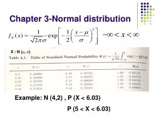
It is often the case that collected data have a distribution with the characteristic shape of the Normal distribution. • Let’s have a look at an example…
Example – Female Haematocrit • Haematocrit measures the percentage of blood volume occupied by packed red blood cells. • Measurements taken from 126 female medical students are as follows…
Female haematocrit measurements 42.0 42.0 40.0 45.0 42.0 43.0 36.0 43.0 40.0 42.0 35.0 46.0 45.0 38.0 40.0 46.0 45.0 43.0 42.0 41.0 44.0 41.0 49.0 42.0 35.0 46.0 44.0 37.0 43.0 42.0 41.0 36.0 41.0 44.0 38.0 40.5 42.0 38.0 35.0 42.0 42.0 40.0 45.0 40.0 55.0 45.0 44.0 44.0 43.0 42.0 42.0 43.0 42.0 45.0 43.0 44.0 41.0 46.0 49.0 44.0 44.0 32.5 42.0 44.0 49.0 41.5 48.0 42.0 39.0 45.0 41.0 42.0 43.0 46.0 40.0 43.0 42.0 44.0 40.0 44.0 41.0 44.0 43.0 49.0 40.5 39.0 48.0 40.0 41.0 41.0 41.0 45.0 36.0 39.0 36.0 38.0 45.0 46.0 41.0 40.0 43.0 34.5 42.0 42.0 39.0 41.5 46.0 42.0 44.0 46.0 44.0 40.0 38.5 40.0 40.0 44.0 39.0 40.0 39.0 43.0 42.0 36.0 46.0 44.5 48.0 45.5 • Let’s look at the shape of the distribution of this data using a histogram…
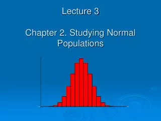
These data show the characteristic shape of the Normal Distribution. • It is characterised by the symmetrical “bell shape”, which corresponds to values near the mean being more common, while values further away “tail off” in terms of their frequencies. • A perfect Normal distribution curve looks like….
In order to understand what it really means for data to be Normally distributed, we first need to consider the idea of probability…
Probability • Probability is used to measure the likelihood of an event occurring. • Definition Suppose we were to repeat a particular experiment over and over again. Then the probability of a particular outcome A is defined as the proportion of the total number of repeats in which A would actually occur, if we were to keep on repeating the experiment. We denote this probability by Pr(A).
Probability Examples 1. Rolling a fair die We roll a standard six-sided die. Let event A be that the die lands with three spots face up. Then the probability of the event A is: Pr(A) = 1/6 ≈ 0.167 because in the long run, the proportion of times that A happens will be 1/6. Note that in this experiment there are six equally likely outcomes, all with probability 1/6.
Probability Examples 2. Tossing a fair coin You toss a fair coin once. Let event A be that the coin lands heads up. Then the probability of the event A is: Pr(A) = ½ = 0.5 because in the long run, the proportion of times that A happens will be 1/2. This time there are two possible outcomes with equal probability. Note that the Probability scale runs between 0 and 1 inclusive. The higher the number, the more likely the event.
Probability Examples 3. Buying a ticket for the UK National Lotto You buy a single ticket for one draw of the UK National Lotto. The event A is that your six numbers exactly match the six main numbers drawn from 1, … , 49, so that you win a share of the jackpot. Then the probability of the event A is: Pr(A) = 1 / 13,983,816 ≈ 0.0000000715 because there are 13,983,816 equally likely outcomes for the six main numbers.
Probability measurements only really make sense for discrete outcomes, i.e. when we can make a list of all the possible outcomes. • When the measurements are on a continuous scale, such as the haematocrit measures, then there are infinitely many possible outcomes, and it is not possible to list them. • The distribution of haematocrit outcomes has roughly the Normal distribution shape: