Download
1 / 43
430 likes | 584 Views
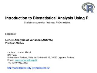
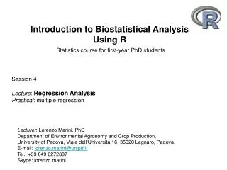
Introduction to Biostatistical Analysis Using R Statistics course for first-year PhD students. Session 4 Lecture : Regression Analysis Practical : multiple regression. Lecturer : Lorenzo Marini DAFNAE, University of Padova, Viale dell’Università 16, 35020 Legnaro, Padova.

E N D
Introduction to Biostatistical AnalysisUsing RStatistics course for first-year PhD students Session 4 Lecture: Regression Analysis Practical: multiple regression Lecturer: Lorenzo Marini DAFNAE, University of Padova, Viale dell’Università 16, 35020 Legnaro, Padova. E-mail: lorenzo.marini@unipd.it Tel.: +39 049 8272807 Skype: lorenzo.marini http://www.biodiversity-lorenzomarini.eu/
Statistical modelling: more than one parameter Nature of the response variable Generalized Linear Models NORMAL POISSON, BINOMIAL … GLM Session 3 General Linear Models Nature of the explanatory variables Categorical Continuous Categorical + continuous ANOVA Regression ANCOVA Session 3 Session 4
REGRESSION REGRESSION Linear methods Non-linear methods Non-linear -One X -Complex relation Simple linear -One X -Linear relation Multiple linear -2 or > Xi - Linear relation Polynomial -One X but more slopes - Non-linear relation
LINEAR REGRESSION lm() Regression analysis is a technique used for the modeling and analysis of numerical data consisting of values of a dependent variable (response variable) and of one or more independent continuous variables (explanatory variables) Assumptions Independence: The Y-values and the error terms must be independent of each other. Linearity between Y and X. Normality: The populations of Y-values and the error terms are normally distributed for each level of the predictor variable x Homogeneity of variance: The populations of Y-values and the error terms have the same variance at each level of the predictor variable x. (don’t test for normality or heteroscedasticity, check the residuals instead!)
LINEAR REGRESSION lm() AIMS 1.To describe the linear relationships between Y and Xi (EXPLANATORY APPROACH) and to quantify how much of the total variation in Y can be explained by the linear relationship with Xi. 2. To predict new values of Y from new values of Xi (PREDICTIVE APPROACH) Xi predictors Y response Yi = α + βxi + εi We estimate oneINTERCEPT and one or moreSLOPES
SIMPLE LINEAR REGRESSION: Simple LINEAR regression step by step: I step: -Check linearity [visualization with plot()] II step: -Estimate the parameters (one slope and one intercept) III step: -Check residuals (check the assumptions looking at the residuals: normality and homogeneity of variance)
SIMPLE LINEAR REGRESSION: Normality Do not test the normality over the whole y
SIMPLE LINEAR REGRESSION MODEL The model gives the fitted values yi = α + βxi SLOPE β = Σ [(xi-xmean)(yi-ymean)] Σ (xi-xmean)2 INTERCEPT α = ymean- β*xmean The model does not explained everything RESIDUALS Residuals= observed yi- fitted yi Observed value
SIMPLE LINEAR REGRESSION Least square regression explanation library(animation) ########################################### ##Slope changing # save the animation in HTML pages ani.options(ani.height = 450, ani.width = 600, outdir = getwd(), title = "Demonstration of Least Squares", description = "We want to find an estimate for the slope in 50 candidate slopes, so we just compute the RSS one by one. ") ani.start() par(mar = c(4, 4, 0.5, 0.1), mgp = c(2, 0.5, 0), tcl = -0.3) least.squares() ani.stop() ############################################ # Intercept changing # save the animation in HTML pages ani.options(ani.height = 450, ani.width = 600, outdir = getwd(), title = "Demonstration of Least Squares", description = "We want to find an estimate for the slope in 50 candidate slopes, so we just compute the RSS one by one. ") ani.start() par(mar = c(4, 4, 0.5, 0.1), mgp = c(2, 0.5, 0), tcl = -0.3) least.squares(ani.type = "i") ani.stop()
SIMPLE LINEAR REGRESSION Parameter t testing Hypothesis testing Ho: β = 0 (There is no relation between X and Y) H1: β ≠ 0 Parameter t testing (test the single parameter!) We must measure the unreliability associated with each of the estimated parameters (i.e. we need the standard errors) SE(β) = [(residual SS/(n-2))/Σ(xi - xmean)]2 t = (β – 0) /SE(β)
SIMPLE LINEAR REGRESSION If the model is significant (β ≠ 0) How much variation is explained? Measure of goodness-of-fit Total SS = Σ(yobserved i- ymean)2 Model SS = Σ(yfitted i - ymean)2 Residual SS = Total SS - Model SS R2 = Model SS /Total SS It does not provide information about the significance Explained variation
SIMPLE LINEAR REGRESSION: example 1 If the model is significant, then model checking 1. Linearity between X and Y? ok No patterns in the residuals vs. predictor plot
SIMPLE LINEAR REGRESSION: example 1 2. Normality of the residuals Q-Q plot + Shapiro-Wilk test on the residuals ok > shapiro.test(residuals) Shapiro-Wilk normality test data: residuals W = 0.9669, p-value = 0.2461 ok
SIMPLE LINEAR REGRESSION: example 1 3. Homoscedasticity Call: lm(formula = abs(residuals) ~ yfitted) Coefficients: Estimate SE t P (Intercept) 2.17676 2.04315 1.065 0.293 yfitted 0.11428 0.07636 1.497 0.142 ok
SIMPLE LINEAR REGRESSION: example 2 1. Linearity between X and Y? no no yes NO LINEARITY between X and Y
SIMPLE LINEAR REGRESSION: example 2 2. Normality of the residuals Q-Q plot + Shapiro-Wilk test on the residuals no > shapiro.test(residuals) Shapiro-Wilk normality test data: residuals W = 0.8994, p-value = 0.001199 no
SIMPLE LINEAR REGRESSION: example 2 3. Homoscedasticity NO YES
SIMPLE LINEAR REGRESSION: example 2 How to deal with non-linearity and non-normality situations? Transformation of the data -Box-cox transformation (power transformation of the response) -Square-root transformation -Log transformation -Arcsin transformation Polynomial regression Regression with multiple terms (linear, quadratic, and cubic) Y= a + b1X + b2X2 + b3X3 + error X is one variable!!!
POLYNOMIAL REGRESSION: one X, n parameters Hierarchy in the testing (always test the highest)!!!! n.s. n.s. n.s. No relation X X + X2 + X3 X + X2 P<0.01 P<0.01 P<0.01 Stop Stop Stop NB Do not delete lower terms even if non-significant
MULTIPLE LINEAR REGRESSION: more than one x Multiple regression Regression with two or more variables Y= a + b1X1 + b2X2+… + biXi Assumptions Same assumptions as in the simple linear regression!!! The Multiple Regression Model There are important issues involved in carrying out a multiple regression: • which explanatory variables to include (VARIABLE SELECTION); • NON-LINEARITY in the response to the explanatory variables; • INTERACTIONS between explanatory variables; • correlation between explanatory variables (COLLINEARITY); • RELATIVE IMPORTANCE of variables
MULTIPLE LINEAR REGRESSION: more than one x Multiple regression MODEL Regression with two or more variables Y = a+ b1X1+ b2X2+…+ biXi Each slope (bi) is a partial regression coefficient: bi are the most important parameters of the multiple regression model. They measure the expected change in the dependent variable associated with a one unit change in an independent variable holding the other independent variables constant. This interpretation of partial regression coefficients is very important because independent variables are often correlated with one another.
MULTIPLE LINEAR REGRESSION: more than one x Multiple regression MODEL EXPANDED We can add polynomial terms and interactions Y= a + linear terms +quadratic & cubic terms+ interactions QUADRATIC AND CUBIC TERMS account for NON-LINEARITY INTERACTIONS account for non-independent effects of the factors
MULTIPLE LINEAR REGRESSION: Multiple regression step by step: I step: -Check collinearity (visualization with pairs() and correlation) -Check linearity II step: -Variable selection and model building (different procedures to select the significant variables) III step: -Check residuals (check the assumptions looking at the residuals: normality and homogeneity of variance)
MULTIPLE LINEAR REGRESSION: I STEP I STEP: -Check collinearity -Check linearity Let’s begin with an example from air pollution studies. How is ozone concentration related to wind speed, air temperature and the intensity of solar radiation?
MULTIPLE LINEAR REGRESSION: II STEP II STEP: MODEL BUILDING Start with a complex model with interactions and quadratic and cubic terms Model simplification Minimum Adequate Model How to carry out a model simplification in multiple regression 1. Remove non-significant interaction terms. 2. Remove non-significant quadratic or other non-linear terms. 3. Remove non-significant explanatory variables. 4. Amalgamate explanatory variables that have similar parameter values.
MULTIPLE LINEAR REGRESSION: II STEP Start with the most complicate model (it is one approach) model1<lm( ozone ~ temp*wind*rad+I(rad2)+I(temp2+I(wind2)) !!!!!! We cannot delete these terms !!!!!!! Delete only the highest interaction temp:wind:rad
MULTIPLE LINEAR REGRESSION: II STEP Manual model simplification (It is one of the many philosophies) Deletion the non-significant terms one by one: Hierarchy in the deletion: 1. Highest interactions 2. Cubic terms 3. Quadratic terms 4. Linear terms COMPLEX Deletion At each deletion test: Is the fit of a simpler model worse? SIMPLE IMPORTANT!!! If you have quadratic and cubic terms significant you cannot delete the linear or the quadratic term even if they are not significant If you have an interaction significant you cannot delete the linear terms even if they are not significant
MULTIPLE LINEAR REGRESSION: III STEP III STEP: we must check the assumptions NO NO Variance tends to increase with y Non-normal errors We can transform the data (e.g. Log-transformation of y) model<lm( log(ozone) ~ temp + wind + rad + I(wind2))
MULTIPLE LINEAR REGRESSION: more than one x The log-transformation has improved our model but maybe there is an outlier
PARTIAL REGRESSION: With partial regression we can remove the effect of one or more variables (covariates) and test a further factor which becomes independent from the covariates WHEN? • Would like to hold third variables constant, but cannot manipulate. • Can use statistical control. • HOW? • Statistical control is based on residuals. If we regress Y on X1 and take residuals of Y, this part of Y will be uncorrelated with X1, so anything Y residuals correlate with will not be explained by X1.
PARTIAL REGRESSION: VARIATION PARTITIONING Relative importance of groups of explanatory variables R2= 76% (TOTAL EXPLAINED VARIATION) What is space and what is environment? Total variation Latitude (km) Space ∩ Envir. Unexpl. Space Environment Longitude (km) Explained variation Full.model<lm(species ~ environment i + space i) Site Response variable: orthopteran species richness Explanatory variable: SPACE (latitude + longitude) + ENVIRONMENT (temperature + land-cover heterogeneity)
VARIATION PARTITIONING: varpart(vegan) Full.model<lm(SPECIES ~ temp + het + lat + long) Unexpl. Environment Space TVE=76% Env.model<lm(SPECIES ~ temp + het) env.residuals Unexpl. Environment Space Pure.Space.model<lm(ENV.RESIDUALS ~ lat + long) VE=15% Unexpl. Environment Space Space.model<lm(SPECIES ~ lat + long) space.residuals Unexpl. Environment Space Pure.env.model<lm(SPACE.RESIDUALS ~ tem + het) VE=40% Unexpl. Environment Space
NON-LINEAR REGRESSION: nls() Sometimes we have a mechanistic model for the relationship between y and x, and we want to estimate the parameters and standard errors of the parameters of a specific non-linear equation from data. We must SPECIFY the exact nature of the function as part of the model formula when we use non-linear modelling In place of lm() we write nls() (this stands for ‘non-linear least squares’). Then, instead of y~x+I(x2)+I(x3) (polynomial), we write the y~function to spell out the precise nonlinear model we want R to fit to the data.
NON-LINEAR REGRESSION: step by step 1. Plot y against x Alternative approach 2. Get an idea of the family of functions that you can fit Multimodel inference (minimum deviance + minimum number of parameters) 3. Start fitting the different models AIC = scaled deviance +2k 4. Specify initial guesses for the values of the parameters k= parameter number + 1 Compare GROUPS of model at a time 5. [Get the MAM for each by model simplification] 6. Check the residuals Model weights and model average [see Burnham & Anderson, 2002] 7. Compare PAIRS of models and choose the best
nls(): examples of function families Asymptotic functions S-shaped functions Humped functions Exponential functions
nls(): Look at the data Asymptotic functions ? S-shaped functions Humped functions Exponential functions Asymptotic exponential Understand the role of the parameters a, b, and c Using the data plot work out sensible starting values. It always helps in cases like this to work out the equation’s at the limits – i.e. find the values of y when x=0 and when x=
nls(): Look at the data Fit the model 1. Estimate of a, b, and c (iterative) 2. Extract the fitted values (yi) 3. Check graphically the curve fitting Can we try another function from the same family? Model choice is always an important issue in curve fitting (particularly for prediction) Different behavior at the limits! Think about your biological system not just residual deviance!
nls(): Look at the data Michaelis–Menten Fit a second model 1. Extract the fitted values (yi) 2. Check graphically the curve fitting You can see that the asymptotic exponential (solid line) tends to get to its asymptote first, and that the Michaelis–Menten (dotted line) continues to increase. Model choice, therefore would be enormously important if you intended to use the model for prediction to ages much greater than 50 months.
Application of regression: prediction Regression models for prediction A model can be used to predict values of y in space or in time knowing new xi values Spatial extent + data range YES NO Before using a model for prediction it has to be VALIDATED!!! 2 APPROACHES
VALIDATION 1. In data-rich situation, set aside validation (use one part of data set to fit model, second part for assessing prediction error of final selected model). Residual=Prediction error Real y Model fit Predicted 2. If data scarce, must resort to “artificially produced” validation sets Cross-validation Bootstrap
Cross-validation estimate of prediction error is average of these K-FOLD CROSS-VALIDATION Split randomly the data in K groups with roughly the same size Take turns using one group as test set and the other k-I as training set for fitting the model 1 2 3 4 5 1. Prediction error1 Test Train Train Train Train 2. Prediction error2 Train Train Test Train Train 3. Prediction error3 Train Train Train Test Train 4. Prediction error4 Train Test Train Train Train 5. Prediction error5 Train Train Train Train Test
BOOTSTRAP 1. Generate a large number (n= 10 000) of bootstrap samples … n=10000 2. For each bootstrap sample, compute the prediction error Error3 … Errorn Error1 Error2 3. The mean of these estimates is the bootstrap estimate of prediction error
Application of regression: prediction 1. Do not use your model for prediction without carrying out a validation If you can, use an independent data set for validating the model If you cannot, use at least bootstrap or cross-validation 2. Never extrapolate