Download
1 / 22
240 likes | 427 Views
Introduction to Biostatistical Analysis Using R Statistics course for PhD students in Veterinary Sciences. Session 5 Lecture : Multivariate analysis Practical : Assessment exercises. Lecturer : Lorenzo Marini, PhD Department of Environmental Agronomy and Crop Production,

E N D
Introduction to Biostatistical AnalysisUsing RStatistics course for PhD students in Veterinary Sciences Session 5 Lecture: Multivariate analysis Practical: Assessment exercises Lecturer: Lorenzo Marini, PhD Department of Environmental Agronomy and Crop Production, University of Padova, Viale dell’Università 16, 35020 Legnaro, Padova. E-mail: lorenzo.marini@unipd.it Tel.: +39 0498272807 http://www.biodiversity-lorenzomarini.eu/
Type of analyses Variables Univariate analysis Y - One Response variable (Y): (e.g. Y= hormone concentration) - One or more explanatory variables (Xi) (e.g. N, pH, Temp) Multivariate analysis Y1 Y2 Y3 Y4 Y5 Variables - More than 1 response variable (Yi) (e.g. Yi= abundance of microbe species in gut or DNA sequences in different individuals) - One or more explanatory variables (xi) (e.g. N, pH, Temp)
MULTIVARIATE ANALYSES Response matrix Explanatory matrix Yes 3. Constrained Ordinations (RDA, CCA…) No explanatory matrix 1. CLASSIFICATION (Cluster Analysis) 2. Unconstrained ORDINATIONS (PCA, CA…)
Dissimilarity Distance-dissimilarity The most natural dissimilarity measure is the Euclidean distance (distance in variable space - each variable is an axis) Sp 1 object3 object 1 Sp 2 object 2 Sp 3 [Σ(xi j-xi k)2]0.5 Euclidean distance: object1-object2= 2 object2-object3= 6 object1-object3= 5 One value for each possible pair of objects
Dissimilarity There are many different dissimilarity indices (e.g.): - Jaccard index - Manhattan - Bray-Curtis - Morisita - 1-Correlation… Source of subjectivity in the choice of the method
CLASSIFICATION: Hierarchical clustering Aim: Clustering is the classification of objects into different groups, or more precisely, the partitioning of a data set into subsets (clusters), so that the data in each subset (ideally) share some common traits - often proximity according to some defined distance measure High subjectivity in both step 1 and step 2 2. Clustering method 1. Distance matrix Hierarchical clustering builds (agglomerative), or breaks up (divisive), a hierarchy of clusters. Agglomerative algorithms begin at the top of the tree, whereas divisive algorithms begin at the root. (In the figure, the arrows indicate an agglomerative clustering.)
CLASSIFICATION: Hierarchical clustering Increasing dissimilarity
CLASSIFICATION: Hierarchical clustering • Main biostatistical applications: • Phylogeny (old methods) • Bioinformatics • In sequence analysis, clustering is used to group homologous sequences into gene families • In genotyping platforms clustering algorithms are used to automatically assign genotypes.
ORDINATION Definition In multivariate analysis, ordination is a method complementary to data clustering, and used mainly in exploratory data analysis (rather than in hypothesis testing). Ordination orders objects that are characterized by values on multiple variables (i.e., multivariate objects) so that similar objects are near each other and dissimilar objects are farther from each other. These relationships between the objects, on each of several axes (one for each variable), are then characterized numerically and/or graphically.
UNCONSTRAINED ORDINATION They order objects according to traits, NO explanatory variables Principal Components Analysis (PCA) PCA is mathematically defined as an orthogonallinear transformation that transforms the data to a new coordinate system such that the greatest variance by any projection of the data comes to lie on the first coordinate (called the first principal component), the second greatest variance on the second coordinate, and so on. PCA assumes linear response curves. Maximization of the variation explained by the axes
UNCONSTRAINED ORDINATION: PCA PCA PCA is theoretically the optimal linear scheme, in terms of least mean square error, for compressing a set of high dimensional vectors into a set of lower dimensional vectors and then reconstructing the original set Total Variance = Σλ n= 1 Original variables x1, x2, x3, ..., xn Components y1 = a1x1 + a2x2+…+ anxn y2 = b1x1 + b2x2+…+ bnxn y3 = c1x1 + c2x2+…+ cnxn λ1=variance1 λ2=variance2 λ3=variance3
UNCONSTRAINED UNCONSTRAINED ORDINATION: PCA Biometry: geographical variation of skull morphology 18 measures on skull + 6 on mandible = 24 response variables 27 Localities (objects)
UNCONSTRAINED UNCONSTRAINED ORDINATION: PCA Biometry 24 measures (variables) 27 Localities (North vs. South) (objects) North 6.8% South 77.6% 7.0% 74.8%
UNCONSTRAINED ORDINATION: PCA Main biostatistical applications: • Reduction of a set of intercorrelated predictors to a smaller set of independent variables in multiple regression • For example, two situations in regression where principal components may be useful are (1) if the number of response variables is large relative to the number of observations, a test may be ineffective or even impossible (e.g. biometry), and (2) if the explanatory variables are highly correlated, the estimates of regression coefficients may be unstable. In such cases, the regression variables can be reduced to a smaller number of principal components that will yield a better test or more stable estimates of the regression coefficients. • 2. Indirect gradient analysis • In the analysis of community data we can do a multiple regression between the PCA axes and some explanatory variables to explain the change in species composition
UNCONSTRAINED VS. CONSTRAINED If you have both the environmental data and the species composition, you can both calculate the unconstrained ordination first and then calculate regression of ordination axes on the measured environmental variables or you can calculate directly the constrained ordination. The approaches are complementary and should be used both! By calculating the unconstrained ordination first you surely do not miss the main part of the variability in species composition, but you could miss the part of variability that is related to the measured environmental variables. By calculating the constrained ordination, you surely do not miss the main part of the variability explained by the environmental variables, but you could miss the main part of variability that is not related to the measured environmental variables.
CONSTRAINED ORDINATION: RDA Explanatory matrix Response matrix Think like you are working on a linear multiple regression model RDA Explanatory matrix Response vector Multiple regression
CONSTRAINED ORDINATION: RDA The unconstrained ordination axes correspond to the directions of the greatest variability within the data set. The constrained ordination axes correspond to the directions of the greatest variability of the data set that can be explained by the environmental variables There are as many constrained axes as there are independent explanatory variables
CONSTRAINED ORDINATION: RDA Assessment to what extent dietary treatment and time (further referred to as environmental variables) affected the ileal microbiota as measured by DGGE profiling
CONSTRAINED ORDINATION: RDA The constrained ordination axes correspond to the directions of the greatest variability of the data set that can be explained by the environmental variables How to choose our explanatory variables? Can we test them? We can use a pseudo-F test using Monte Carlo Permutation
MONTE CARLO PERMUTATION F value = 10 RDAreal First permutation F1 value = 1.4 RDA1 Repeat for n times Get n F values Compute the pseudo F Fixed Shuffle
How to prepare the report Report is composed of two parts: abstract + R script Abstract layout: A4 Font 11 Margins (2.5 cm) Times new roman Word count: no more than 1000 words Lines numbered Double lines 1 figure with caption and/or 1 table with caption Four sections: 1. Title: give a title to your study 2. Introduction: just set the aims of the study 3. Material and Methods: explain the sampling & statistical analysis performed 4. Results and Discussion: present the results with 1 figure and/or 1 table and discuss briefly.
How to prepare the report R script Write down the script used to perform the analysis on a separate page. Include everything you used. You can find all you need in the single practical we have done. Topic: multiple regression or ANOVA If you are in trouble look at these books how to run your analysis (http://cran.r-project.org/): Practical Regression and Anova using R” by Julian Faraway Statistics Using R with Biological Examples” by Kim Seefeld and Ernst Linder An Introduction to R: Software for Statistical Modelling & Computing” by Petra Kuhnert and Bill Venables