Download
1 / 44
440 likes | 472 Views
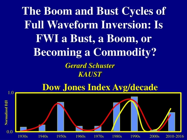
This article explores the history, examples, and challenges of Full Waveform Inversion (FWI), a seismic imaging technique. It discusses the boom and bust cycles it has undergone and its potential future as a commodity.

E N D
The Boom and Bust Cycles of Full Waveform Inversion: Is FWI a Bust, a Boom, or Becoming a Commodity? Gerard Schuster KAUST Dow Jones Index Avg/decade 1.0 Normalized DJI 0.0 1930s 1940s 1950s 1960s 1970s 1980s 1990s 2000s 2010-2016
Outline 1. Inversion Overview: Lm = d 1 1 Lm = d 2 2 2. Seismic Experiment: Lm = d . . N N . 3. FWI, History, Examples L d 1 1 m = L d 2 2 4. Summary
Medical vs Seismic Imaging CAT Scan MRI Full Waveform Inversion Tomogram
Traveltime Tomogram & Migration Images t time t Vshallow = L/t L L Vdeep = L/t
Traveltime Tomogram & Migration Images time Vshallow = L/t Intersection of down & up rays Vdeep = L/t
Traveltime Tomogram & Migration Images time Vshallow = L/t Vdeep = L/t
Traveltime Tomogram & Migration Images Problems: Hi-Freq. ray tracing, picking traveltimes, tedious, low resolution, fails in complex earth models Shot gather = d(x,t) time Vshallow = L/t migration image Vdeep = L/t
Full Waveform Inversion - Given: d(x,t) = predicted traces Find: v(x,y,z) minimizes e=S[d(x,t)-d(x,t)obs]2 x,t predicted observed residual = Time Problems: Hi-Freq. ray tracing, picking traveltimes, tedious, low resolution, fails in complex earth models
Outline 1. Inversion Overview: Lm = d 1 1 Lm = d 2 2 2. Seismic Experiment: Lm = d . . N N . 3. FWI, History, Examples L d 1 1 m = L d 2 2 4. Summary 4. Summary and Road Ahead
Gulf of Mexico Seismic Survey 4 d Predicted data Observed data 1 Time (s) Goal: Solve overdetermined System of equations for m Lm = d 1 1 0 Lm = d 6 X (km) 2 2 Lm = d . . N N . m
Outline 1. Inversion Overview: Lm = d 1 1 Lm = d 2 2 2. Seismic Experiment: Lm = d . . N N . 3. FWI, History, Examples L d 1 1 m = L d 2 2 4. Summary 4. Summary and Road Ahead
Reflectivity or velocity model Details of Ldm= d-dobs dm(k) = LT(d-dobs)(k) Time (s) 0 dobs 6 X (km) [ ] -1 [ ] d(g|s) = - Predicted data Observed data 2 2 m 1 d2 – 1 d2 d(g|s) = F F c2 dt2 c2 dt2
L= & d = Conventional FWI Solution L d 1 1 L d Given: Lm=d 2 2 In general, huge dimension matrix Find: m s.t. min||Lm-d|| 2 Solution: m = [L L] L d -1 T T or if L is too big m = m – aL (Lm - d) (k+1) (k) (k) T (k) = m – aL (L m - d ) (k) [ ] T + L (L m - d ) T 1 1 1 2 2 2 Problem: L is too big for IO bound hardware
Outline 1. Inversion Overview: Lm = d 1 1 Lm = d 2 2 2. Seismic Experiment: Lm = d . . N N . 3. FWI, History, Examples L d 1 1 m = L d 2 2 4. Summary 4. Summary and Road Ahead
Dow Jones Index vs FWI Index Dow Jones Industrial Avg/decade FWI Index Avg/decade 18.0 0.0 1930s 1940s 1950s 1960s 1970s 1980s 1990s 2000s 2010-2016 Tarantola + French School Bunks Multiscale Exxon+ BP+Pratt Mora
Dow Jones Index vs FWI Index FWI Index Avg/decade 18.0 0.0 1930s 1940s 1950s 1960s 1970s 1980s 1990s 2000s 2010-2016
What Caused the 1st FWI Boom? FWI Index Avg/decade 18.0 0.0 1930s 1940s 1950s 1960s 1970s 1980s 1990s 2000s 2010-2016 FWI v(x,z) True v(x,z) 0 Z (km) 2 0 X (km) 4 0 X (km) 4
What Caused the 1st FWI Bust? FWI Index Avg/decade 18.0 0.0 1930s 1940s 1950s 1960s 1970s 1980s 1990s 2000s 2010-2016 FWI v(x,z) True v(x,z) 0 Z (km) 2 0 X (km) 24 0 X (km) 24
What Caused the 1st FWI Bust? FWI Index Avg/decade 18.0 0.0 1930s 1940s 1950s 1960s 1970s 1980s 1990s 2000s 2010-2016 observed residual predicted 1 5.0 - = Time (s) Waveform Misfit 0.0 0 x Vstart Vtrue V
What Caused the 1st FWI Bust? FWI Index Avg/decade 18.0 0.0 1930s 1940s 1950s 1960s 1970s 1980s 1990s 2000s 2010-2016 observed residual predicted 1 5.0 - = = Time (s) Waveform Misfit 0.0 0 x Vstart Vtrue V
What Caused the 1st FWI Bust? FWI Index Avg/decade 18.0 0.0 1930s 1940s 1950s 1960s 1970s 1980s 1990s 2000s 2010-2016 observed residual predicted Gradient opt. gets stuck local minima 1 5.0 - = = Time (s) Waveform Misfit 0.0 0 x Vstart Vtrue V
How to Cure the 1st FWI Bust? FWI Index Avg/decade 18.0 0.0 1930s 1940s 1950s 1960s 1970s 1980s 1990s 2000s 2010-2016 observed residual predicted 1 5.0 Low-pass filter - = = Time (s) Waveform Misfit Gradient opt global minima 0.0 0 x Vstart Vtrue V
How to Cure the 1st FWI Bust? FWI Index Avg/decade 18.0 0.0 1930s 1940s 1950s 1960s 1970s 1980s 1990s 2000s 2010-2016 observed residual predicted Multiscale FWI v(x,z) 1 5.0 Window early events - = = Time (s) Waveform Misfit 0.0 0 x Vstart Vtrue V
How to Cure the 1st FWI Bust? 2004 EAGE Meeting Started New Boom FWI Index Avg/decade 18.0 0.0 1930s 1940s 1950s 1960s 1970s 1980s 1990s 2000s 2010-2016 Multiscale FWI v(x,z) FWI v(x,z) True v(x,z) 0 Z (km) 2 0 X (km) 24 0 X (km) 24
Outline 1. Inversion Overview: Lm = d 1 1 Lm = d 2 2 2. Seismic Experiment: Lm = d . . N N . 3. FWI, History, Examples: Transmission FWI Norway L d 1 1 m = L d 2 2 4. Summary 4. Summary and Road Ahead
Transmission 3D FWI Norway Marine Data 2300 buried hydrophones, 50,000 shots, sea bottom 70 m 16 km 8 km gas 4.5 Gas cloud 1.5 km/s 3.5 km/s Small dimensions of structures such as sandy outwash channels to 175m depth (Figure 1c) and the scars left on the sea paleo-bottom by drifting icebergs to 500m depth (Figure 1d). A wide low speed region defines the geometry of the gas cloud (Figure 1a, e) the periphery of which a fracture network is identified (Figure 1b, e). The image of a deep reflector, defining the base of the Cretaceous chalk under the tank (Figure 1a, b, white arrows), is uniquely identifiable despite the screen formed by the overlying gas cloud that opposes penetration seismic wave. S. Operto, A. Miniussi, R. Brossier, L. Combe, L. Metivier, V. Monteiller, Ribodetti A., and J. Virieux, 2015, GJI.
Transmission 3D FWI Norway Marine Data 2300 buried hydrophones, 50,000 shots, sea bottom 70 m 16 km 8 km 4.5 gas 1.5 km/s 3.5 km/s
2D FWI R+T Gulf of Mexico Marine Data Transmission 3D FWI Norway Marine Data 2300 buried hydrophones, 50,000 shots, sea bottom 70 m Transmissions 10x stronger than reflections Therefore gradients will spend greater effort updating shallow v(x,y,z) Vshallow Vshallow Vshallow Vdeep ??????
Outline 1. Inversion Overview: Lm = d 1 1 Lm = d 2 2 2. Seismic Experiment: Lm = d . . N N . 3. FWI, History, Examples: R+T FWI Gulf of Mexico L d 1 1 m = L d 2 2 4. Summary 4. Summary and Road Ahead
2D FWI R+T Gulf of Mexico Marine Data Transmission Cigars observed Reflection Rabbit Ears predicted predicted Abdullah AlTheyab (2015)
2D FWI R+T Gulf of Mexico Marine Data R+T Transmission Cigars 0.0 observed Z (km) Migration Image with FWI V(x,z) 3.6 19 0.0 X (km) Migration Image with Initial V(x,z) Migration Image with FWI V(x,z) predicted Abdullah AlTheyab (2015)
Outline 1. Inversion Overview: Lm = d 1 1 Lm = d 2 2 2. Seismic Experiment: Lm = d . . N N . 3. FWI, History, Examples: Phase FWI Surface Waves L d 1 1 m = L d 2 2 4. Summary 4. Summary and Road Ahead
2D KSA Potash Model Test True Model m/s Start Model m/s 0 30 800 600 400 800 600 400 800 600 400 800 600 400 0 30 z (m) z (m) 0 60 120 x(m) 10 m 0 60 120 x(m) surface waves 1D Vs Tomogram m/s WD Vs Tomogram m/s z (m) z (m) 0 30 0 30 0 60 120 x(m) 0 60 120 x(m)
Problem & Solution Z (m) True model 1D Vs Tomogram 0 30 0 30 Problem: 1D Dispersion inversion assumes layered medium (Xia et al. 1999). Dispersion Curves CSGs Radon 1D Inversion Z (m) t(s) Solution: v(x,y,z) minimizes e=S[c(k,w)-c(k,w)obs]2 (Li & Schuster, 2016) Z (m) Z (m) (Radon Transform) FWI: e=S[d(x,t)-d(x,t)obs]2 Dispersion Curves CSGs 0 60 120 x(m) 0 60 120 x(m) x (m) x (m) Radon 1D Inversion C (m/s) t(s) 2D WD WD Vs Tomogram v (m/s) v (m/s) 0 30 C(m/s) Z (m) w(Hz) w(Hz) 0 60 120 x(m)
Seismic Imaging of Olduvai Basin Kai Lu, Sherif Hanafy, Ian Stanistreet, Jackson Njau, Kathy Schick ,Nicholas Toth and Gerard Schuster
The Fifth Fault Olduvai, Tanzania Seismic Data COG 0 0.6 z (m) The Fifth Fault The Fifth Fault m/s 0 500 1000 1500 2000 2500 3000 3500 P-wave Velocity Tomogram Tomogram z (m) 3500 2000 1500 0 0.6 m/s z (m) S-wave Velocity Tomogram (WD) 0 500 1000 1500 2000 2500 3000 3500 0 0.6 1000 800 600 0 500 1000 1500 2000 2500 3000 3500
Summary Multiscale+Skeletonized FWI: e =S |di –dipred |2 v(x,y,z), r(x,y,z) i 2. History 1930s 1980 1990 2010-2016 3. Is FWI a commodity? Almost according to 2 industry experts Is FWI a black box? Not yet, works ~80% time (2 experts) Challenges? Deeper imaging, CPU cost, multiparameter
Summary 4. Road Ahead 3D Elastic Inversion & Adaptive Grid. Worth it? 3D Viscoelastic Inversion. Worth it? Clever Skeletonized FWI Anisotropic Inversion Multiples???? Inversion Deeper than src-rec offset/depth<2
Summary (We need faster migration algorithms & better velocity models) Stnd. FWI Multsrc. FWI IO 1 vs 1/20 or better Cost 1 vs 1/20 or better Sig/MultsSig ? Resolution dx 1 vs 1
P-wave Tomogram 1D S-wave Tomogram 2D WD S-wave Tomogram Qademah Fault, Saudi Arabia Field Data
Comparison of 2D WD Inversion with FWI Start Model FWI of Surface Waves Easy to get stuck in a local minimum (Solano, et al., 2014). A shot gather Vs True Model Vs Tomogram FWI FD t (s) z (m) z (m) x (m) 2D WD of Surface Waves x (m) x (m) Avoid local minimum and apply in 2D/3D model. Vs Tomogram WD Dispersion curve v (m/s) t (s) z (m) x (m) f (Hz) x (m)
How to Cure the 1st FWI Bust? 2004 EAGE Meeting Started New Boom FWI Index Avg/decade 18.0 0.0 1930s 1940s 1950s 1960s 1970s 1980s 1990s 2000s 2010-2016 Multiscale FWI v(x,z) FWI v(x,z) True v(x,z) 0 Z (km) 2 0 X (km) 24 0 X (km) 24
Full Waveform Inversion Given: d(x,t) = Find: v(x,y,z) minimizes e=S[d(x,t)-d(x,t)obs]2 x,t time Vshallow = L/t migration image Vdeep = L/t
Transmission 3D FWI Norway Marine Data 2300 buried hydrophones, 50,000 shots, sea bottom 70 m 16 km 8 km gas 4.5 Gas cloud 1.5 km/s 3.5 km/s Small dimensions of structures such as sandy outwash channels to 175m depth (Figure 1c) and the scars left on the sea paleo-bottom by drifting icebergs to 500m depth (Figure 1d). A wide low speed region defines the geometry of the gas cloud (Figure 1a, e) the periphery of which a fracture network is identified (Figure 1b, e). The image of a deep reflector, defining the base of the Cretaceous chalk under the tank (Figure 1a, b, white arrows), is uniquely identifiable despite the screen formed by the overlying gas cloud that opposes penetration seismic wave. S. Operto, A. Miniussi, R. Brossier, L. Combe, L. Metivier, V. Monteiller, Ribodetti A., and J. Virieux, 2015, GJI.


