Download
1 / 54
550 likes | 710 Views
Climate applications of Ground-Based GPS KNMI 1.12 2003. Professor Lennart Bengtsson ESSC, University of Reading MPI for Meteorology, Hamburg. Water vapour is the dominant greenhouse gas and enhances climate warming significantly

E N D
Climate applications of Ground-Based GPS KNMI 1.12 2003 Professor Lennart Bengtsson ESSC, University of Reading MPI for Meteorology, Hamburg
Water vapour is the dominant greenhouse gas and enhances climate warming significantly Substantial change (+40%) is expected during this century Why do we need to monitor water vapour?
The role of the water cycle in the climate system Precipitation is crucial for life on the planet The largest warming factor of the atmosphere is through the relaease of latent heat amounting to 80-90 WM-2 The net transport of water from ocean to the land surfaces amounts to some 40000 km3/year Precipitation over land is about 3 times as high Water vapour is the dominating greenhouse gas. Removing the effect of water vapour in long wave radiation reduces climate warming at 2 x CO2 by a factor of more than 3. (For the GFDL model from 3.38 K to 1.05 K).
Annual mean global values of relative humidity f (in %) vertically averaged for 850-300 hPa and vertically integrated absolute humidity q (in kg/m2).
Onsala, Sweden Es = 0.13 mm Elgered
Summer 1995-2000 Trends Winter
Integrated Water vapour 1978-1999 ECHAM5: T106/L31 using AMIP2 boundary conditions Preliminary results: Globally averaged results vary between 25.10 mm (1985) and 26.42 mm (1998) Mean value for the 1990s is 1% higher than in the 1980s Interannual variations are similar as in ERA-40 Variations follow broadly temperature observations from MSU (tropospheric channel) under unchanged relative humidity (1°C is equivalent to some 6%).
How has atm. water vapour varied over the last 50 years? Objective: to extend estimates of IWV for longer time periods (Re-analyses exists now for some 55 years)
Questions: 1. How well can we determine IWV from GCM forced by observed SST? 2. How well can we determine it from analyses with observations typical of the pre-satellite period? 3. How well can we determine it from the present observing and assimilation systems?
We have mimicked earlier observing systems by redoing the ERA-40 assimilation for limited periods. This has been done at the ECMWF computer system from ESSC at Reading University Methodology
ERA-40: + 0362 mm IWV/TLT: 3.15 mm/C ( presumably only half as much) ECHAM 5 (1979-1999): + 0.290 mm IWV/TLT: 1.54 mm/C NCEP/NCAR: - 0.056 mm IWV Decadal trend1979-2001
1. ERA 40 - all humidity observations 2. Exp 1 - all space observations 3. Exp 2 - all upper air observations 4. Exp 1 - all upper air observations We have done four main experiments
DJF 1990/1991 JJA 2000 DJF 2000/2001 Experimental periods
1. ERA-40 dry (b02d) 2. No space observations (b03v) (NOSAT) 3. Surface observations only (b046) 4. Space observations only (b040) We call the experiments:
ERA-40 IWV/TLT : 2.85 mm/C ( 4.05 mm/C) ERA 40 (corr) IWV/TLT : 1.55 mm/C IWV Decadal trends1958-2001
ERA-40: + 0.405 mm ERA 40 (corr) : + 0.155 mm ( ERA-40(24.9mm) - NOSAT (23.8mm) = -4.3%) NCEP/NCAR: - 0.238 mm IWV Decadal trends1958-2001
GPS data from global IGS network 1997 - present
How well does the ECMWF operational forecasting system analyse IWV as compared to those retrieved from GPS measurements? To what extent is it possible to separate errors in model analysed IWV from IWV obtained from GPS measurements? What are the most likely sources of errors? What are the long term requirements for a GPS-based water vapour monitoring system?
Comparing operationally analysed IWV and IWV calculated from surface based GPS measurements 1. Calculate IWV from GPS signal delay (temperatures from ECMWF operational analyses and pressure from the GPS station or if not available interpolate from met stations) (Care must be taken in the vertical interpolation of moisture due to the fact that the model height differs from station height)
Determination of integrated water vapour, IWV Methodology Zenith path delay, ZPD, from GPS measurements Obtain temperature from operational weather prediction model Surface pressure from met. observations Calculate IWV
Error estimates Measurement error: co-located GPS stations (mid-latitudes) indicate very small errors (<0.7 mm IWV) Horizontal interpolation error: (<100 km) and small vertical interpolation (<200 m) also indicate small errors (<0.6mm)
Results We undertook intercomparison between IWV analyses and GPS calculated GPS for Jan. and Jul. 2000 and 2001. For all stations we calculated the standard deviation of the daily differences (SD) and the monthly average difference (bias) . 1. When both SD and bias were small we concluded that both GPS and the analyzed fields were reliable with an error of the same order as the difference between the estimates.
Results 2. When both SD and bias are large it is generally not possible to conclude whether the GPS measurements or the analyzed values are incorrect or both. However, a detailed inspection of the daily differences can be helpful. 3. When SD is large and the bias is small then we may conclude that it is more likely that GPS is more reliable than the analyzed value. 4. When SD is small and the bias large then we may conclude that it is more likely that the analyzed values are more accurate then the GPS.
January 2001: IWV [mm] for station Gough Island (South Atlantic)
January 2001: Vertical humidity profile from radiosonde measurements and OA at station Quad City (Iowa, USA) OA
July 2001: Vertical humidity profile from radiosonde measurements and OA at station Quad City (Iowa, USA) OA
January 2000: IWV [mm] for station Ascension (Trop. Atlantic)
July 2000: IWV [mm] for station Ascension (Tropical Atlantic)
Regional station averages of normal. bias (GPS- OA) (IWV bias divided by GPS derived IWV) in %
Regional station averages of normal. bias (GPS- ERA 40) (IWV bias divided by GPS derived IWV) in %