Download
1 / 60
600 likes | 795 Views
VIII. Introduction to Response Surface Methodology Sequential Experimentation 1. Phases of Experimentation. I. Screening very small design (Resolution III) little, if any, replication analyze by normal probability plots extremely cost conscious (save resources for later)

E N D
VIII. Introduction to Response Surface Methodology • Sequential Experimentation • 1. Phases of Experimentation
I. Screening • very small design (Resolution III) • little, if any, replication • analyze by normal probability plots • extremely cost conscious (save resources for later) • little, if any, concern about lack-of-fit • II. Initial Steepest Ascent (Descent) • replicate at least the center • begin to be concerned over lack-of-fit • serious consideration to Resolution IV or higher designs • less cost conscious
III. Follow-Up Steepest Ascent • IV. Optimization • replication extremely important • often starts as a mid-course correction • lack-of-fit may suggest design augmentation • popular designs • (a) central composite design (CCD) • (b) augment to a CCD • (c) Box-Behnken • extremely expensive
Important Considerations in Choosing Designs • Purpose of Experiment • Proposed Model • Estimation versus Testing • Concern Over Lack-of-Fit • Ability to Augment, if Necessary • Protection from Outliers
The Relationship Between Design and Model The specific design used determines which models are estimable! 1. Screening Designs 2. “Interactive” Model
B. Steepest Ascent Steepest ascent is an example of an optimization. In calculus, how do we optimize something? Consider a situation where we may model the response by a strict first-order model Taking the first derivative with respect to xj,
Technically, we find the path of steepest ascent by a constrained optimization technique based on Lagrangian multipliers. If we have only two factors, the path of steepest ascent is the line from the origin to the maximum response over the circle defined by where c is the radius of the circle. For k ≥ 3 factors, the path of steepest ascent is the line from the origin to the maximum response over the sphere defined by
Since the path of steepest ascent represents the optimum response over spheres, we need to construct this path in the metric where spheres make the most sense. • Our procedure is: • construct the path in the design variables, and • convert this line back to the natural units.
Let x1 be the “key” factor, and let x10 be a specific value for this factor along the desired path. • The settings for the other factors are • This path passes through the center of the region of interest. • To convert this line back to the natural units, • let cj be the center value, in the natural units, for the jth factor, and • let dj be the “scaling” factor. • Let be the specific setting for the jth factor along the path of steepest ascent; thus,
We usually pick the factor with the largest in absolute value estimated coefficient as our key factor. We construct the line by increasing this key factor by a convenient amount each time. We then run a series of experiments along this path. Example: Kilgo (1988) performed an experiment to determine the effect of CO2 pressure, CO2 temperature, peanut moisture, CO2 flow rate and peanut particle size on the total yield of oil per batch of peanuts. A 25-1design was carried out and only temperature, x2, and particle size, x5, were important.
Since x5 has the largest in absolute value coefficient, we use it as our key factor. For a specific setting of particle size, x50, along the path, the appropriate setting for temperature, x20, is given by We can convert each value of x20 back to the natural units by
We can convert each value of x50 back to the natural units by
C. Second-Order Experiments • 1. Overview • For first order designs, we must have: • at least two levels for each variables. • at least as many points as parameters to estimate, ie $k+1$; and • the main effects can not be completely aliased with each other • For a second order model, we now must have: • at least three levels for each variable in order to estimate both the first order and pure quadratic effects; • at least as many points as parameters to estimate, ie • the main effects and two factor interactions cannot be completely aliased with each other.
The first design which meets these criteria is the 3k factorial design. • Note: • this design uses three levels for each variable. • 3k ≥ (k+1)(k+2)/2 [equality if and only if k=1] • the 3k allows us to estimate all first order, pure quadratic, two-factor and higher interactions. • A major disadvantage of the 3k factorial: • Often the 3k design points are more than are required for the second order model. • Thus, the 3k factorial is really too expensive to be practical.
2. The Central Composite Design • The single most popular second order response surface design is the central composite design (CCD) developed by Box and Wilson (JRSS, B 1951). • The CCD was intended to be a more economical alternative to the 3k. • The design consists of three parts: • a Res. V fraction of a 2k; • a series of “axial” runs; and • a series of center runs.
Sometimes, we convey this information by: Note: The CCD is rather flexible in that is not fixed. Thus, we may choose in order to meet some particular needs.
It is instructive to see the two variable (k=2) CCD with Note: With the center run, the k=2 CCD with is the 32 factorial design.
For k = 3, the CCD is Note: With a single center run, the CCD requires 15 design runs [23 + 2•3 + 1] as opposed to the 27 required by a 33 factorial.
There are three common choices for $\alpha$: • 1 (cuboidal) • (spherical ccd) • (rotatable) where nf is the number of factorial points. • A rotatable design is one where the prediction variance for any two points the same distance from the design center is the same. • As a result, if a design is rotatable, the prediction variance at some specific location only depends on that location's distance from the design center.
Finally, an important question concerns how many center runs should we use. From a variance-based optimality perspective: 1-3 are usually enough. For detecting Lack of Fit, probably 6-8.
D. Optimization • Primary goal: of the second order experiment: optimization. • Consider: • From calculus, the point of optimal response is • either the stationary point • or some point on the boundary of the region. • Let x0 denote the factor settings at the stationary point. • Let y0 be the response at this point. • To find x0, we need to solve the system obtained by
It is important to note that the stationary point may be: • a point of maximum response; • a point of minimum response, or • a saddle point. • Even if the stationary point is an optimum, it may lie outside the region of experimentation. • Hence, we have little faith in it. • Bottom Line: Often, the stationary point is not a reliable point of optimal response. • Thus, the point of optimal response often lies on the boundary of the region of interest.
How should we find this point? Consider Lagrangian multipliers. We thus optimize Subject to the constraint that where R is the radius of the region of interest. Let where μ is the Lagrangian multiplier.
D. Multiple Responses • In many engineering experiments, we have more than one response of interest. • The key: to find appropriate compromise operating conditions. • Two basic approaches for jointly optimizing two or more responses: • the desirability function, and • nonlinear programming approaches. • Several statistical software packages include some form of the desirability function. • Some spreadsheets, including EXCEL, use good reduced gradient algorithms to perform appropriate constrained optimization.
The Desirability Function • The desirability function provides an overall measure for the “goodness” of a specific setting: • A large value indicates a desirable set of values for the various responses. • A low value indicates an undesirable set of values. • Derringer and Suich (Journal of Quality Technology 1980) proposed an approach which: • 1. determines the individual desirabilities for each response and • 2. then combines these individual desirabilities into an overall desirability. • The analyst then seeks to find the settings in the factors which maximize the overall desirability.
The individual desirabilities depend upon whether we wish • to maximize the response of interest, • to minimize the response of interest, or • to achieve a specific target value for the response of interest. • Derringer and Suich use a scale from 0, which represents completely undesirable, to 1, which represents fully desirable, for their individual desirability functions. • Consider the target value case first. • is the predicted value for the response. • yT is the specific target value for the response of interest. • yL is the smallest possible value which has any desirability. • yU is the largest possible value which has any desirability.
One approach defines the desirability for this response by • With this definition, • we give any predicted value for the response less than yL or greater than yU a desirability of 0. • if the predicted value is exactly at the target value, we give it a desirability of 1. • the further the predicted value is from the target, the lower desirability we give it.
Derringer and Suich actually proposed the following slight modification
The exponents s and t provide greater flexibility in assigning the desirability within the range of interest.
Suppose we wish to maximize the response. • yL is the smallest desirable value for this response. • yU is a fully desirable value. • Basically, yU represents the point of diminishing returns. • In some cases, yU represents a true bound for the response. • In other cases, yU is some arbitrary value larger than the largest • observed response.
Suppose we wish to minimize the response. • yU is the largest desirable value for this response. • yL is a fully desirable value. • Basically, yL represents the point of diminishing returns.
Once we have the individual desirabilities, we need to combine them in a meaningful way. • How should we do this? • Note: • If any of the individual responses is completely undesirable, then the overall desirability also should be completely undesirable. • Similarly, the overall desirability should be 1 if and only if all of the individual responses are completely desirable. • Suppose we have m responses of interest. • Let d1, d2, … , dm be the individual desirabilities. • Derringer and Suich defined the overall desirability, D, by • which is the geometric mean of the desirabilities.
Myers and Montgomery (1995) outline an experiment, originally presented in Box, Hunter, and Hunter (1978). • Purpose: to find the settings for • reaction time (x1), • reaction temperature (x2), and • the amount of catalyst (x3) • which maximize the conversion (y1) of a polymer and achieves a target value of 57.5 for the thermal activity (y2). • The lower bound for the conversion is 80. • The maximum possible value is 100. • Thermal activity must be between 55 and 60.
A reasonable model for conversion is A reasonable model for thermal activity is
Let • s=1 for conversion and • s=t=1 for thermal activity. • The Derringer-Suich approach recommends a setting of • This setting gives a predicted conversion of 95.21 and a predicted thermal activity of 57.50. • The overall desirability for this setting is 0.8720, which is reasonably close to 1.
Nonlinear Programming Approaches Jointly optimizing two or more responses when the prediction equations contain second order or higher terms is a standard example of a nonlinear programming problem. Many spreadsheets have built-in routines for solving these problems, for example the SOLVER routine in Microsoft EXCEL. The major spreadsheets use good algorithms, usually based on reduced gradients. We simply need 1. to input the appropriate prediction equations, 2. to input the constraints, and 3. to specify one response as the ``key.'' The spreadsheet routine finds the optimal setting.
These routines are not guaranteed to find a solution within the experimental region unless we specify some additional constraints. For cuboidal experimental regions, i.e. when we use a face centered cube CCD, then each xj must fall within the interval -1 to 1. In which case, we need the following additional constraints: For spherical experimental regions, we need the additional constraint With these additional constraints, the spreadsheet routine may not find a feasible solution. When this occurs, we must relax one or more of our constraints in order to find a solution.
We can use the SOLVER routine in Microsoft EXCEL to find optimal conditions. We use the same second order prediction equations as before. Recall, we seek to maximize the conversion. We thus specify conversion, , as our key response and tell the routine that we want to maximize it. Since we have a target value of 57.5 for the thermal activity, we specify the following constraint: Since this experiment uses a spherical CCD, we need to impose the additional constraint
The spreadsheet recommends the setting This setting gives a conversion of 94.37% and a thermal activity of 57.5.
E. Robust Parameter Design • 1. Overall Taguchi Philosophy • Consider the manufacture of a ball point pen. • important characteristic is the fit between the barrel and the cap. • barrel and the cap are produced by separate injection molding processes. • How can we produce these barrels and caps such that the fit is “optimal”? • What are the real issues in this problem?
The Japanese would view any part which does not achieve the target value as having some tangible loss of value. Often, they use a squared error loss function: Thus, a part may be within specifications and still considered “poor”, just not quite poor enough to be rejected. Impacts of such a philosophy 1. should seek conditions which minimize the expected “loss” 2. must consider both the mean and the variance
2. Overview of Taguchi's Parameter Design Fundamental to this approach are the concepts of 1. control factors --- factors which the experimenter can readily control. 2. noise factors • factors which the experimenter either cannot or will not directly control in the process • factors “move” randomly in actual process although they can be fixed for the experiment. Suppose we wish to develop a cake mix “robust” to customer use. What are possible control factors? What are possible noise factors?
Goal of parameter design: find the settings for the control factors which are most “robust” to the noise factors. Taguchi proposes “crossing”: 1. a design for the control factors (inner or control array) 2. a design for the noise factors (outer or noise array) Each point of the inner array is replicated according to a design in the noise factors called the outer array. Typically, these designs are “saturated” or “near-saturated”. For example, suppose we have three control and three noise factors. Let x1, x2, and x3 represent the control factors. Let z1, z2, and z3 represent the noise factors.
An appropriate inner array is a 23-1 fraction or x1 x2 x3 -1 -1 -1 -1 1 1 1 -1 1 1 1 -1 Each of these settings is replicated by the outer array. z1 z2 z3 -1 -1 -1 -1 1 1 1 -1 1 1 1 -1
The resulting design consists of 4 x 4 or 16 runs and follows. x1 x2 x3z1 z2 z3 -1 -1 -1 -1 -1 -1 -1 1 1 1 -1 1 1 1 -1 -1 1 1 -1 -1 -1 -1 1 1 1 -1 1 1 1 -1 1 -1 1 -1 -1 -1 -1 1 1 1 -1 1 1 1 -1 1 1 -1 -1 -1 -1 -1 1 1 1 -1 1 1 1 -1
While the inner and outer arrays are completely saturated, all of the interactions between the control and noise factors are estimable! • An important question: • Why run the experiment in the noise factors? • We seek to find the settings in the control factors which are most “robust” to the noise factors. • Thus, the noise levels ±1 correspond to what? • What is the natural consequence? • How does this contrast with typical experimentation?
All the designs recommended by Taguchi (the so-called “Taguchi designs”) are orthogonal arrays of strength 2. • allow the estimation of “main effects” • do not allow the estimation of any interactions. • Examples of orthogonal arrays of strength 2 include: • 1. Resolution III fractional factorial designs • 2. Plackett-Burman designs. • Three level orthogonal arrays do exist. • allow the estimation of the linear and pure quadratic terms • do not allow estimation of the two-factor or higher interactions.