Active Random Fields
Active Random Fields. Adrian Barbu. The MAP Estimation Problem. Estimation problem: Given input data y, solve Example: Image denoising Given noisy image y , find denoised image x Issues Modeling : How to approximate ? Computing : How to find x fast?. Noisy image y.

Active Random Fields
E N D
Presentation Transcript
Active Random Fields Adrian Barbu
The MAP Estimation Problem • Estimation problem: Given input data y, solve • Example: Image denoising • Given noisy image y, find denoised image x • Issues • Modeling: How to approximate ? • Computing: How to find x fast? Noisy image y Denoised image x
MAP Estimation Issues • Popular approach: • Find a very accurate model • Find best optimum x of that model • Problems with this approach • Hard to obtain good • Desired solution needs to be at global maximum • For many models , the global maximum cannot be obtained in any reasonable time. • Using suboptimal algorithms to find the maximum leads to suboptimal solutions • E.g. Markov Random Fields
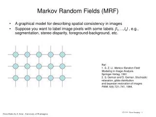
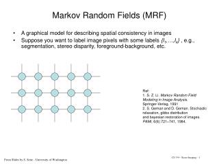
Markov Random Fields • Bayesian Models: • Markov Random Field (MRF) prior • E.g. Image Denoising model • Gaussian Likelihood • Fields of Experts MRF prior • Differential Lorentzian • Image filters Ji Image Filters Ji Roth and Black, 2005
MAP Estimation (Inference) in MRF • Exact inference is too hard • For the Potts model, one of the simplest MRFs it is already NP hard (Boykov et al, 2001) • Approximate inference is suboptimal • Gradient descent • Iterated Conditional Modes (Besag 1986) • Belief Propagation (Yedidia et al, 2001) • Graph Cuts (Boykov et al, 2001) • Tree-Reweighted Message Passing (Wainwright et al, 2003)
Gradient Descent for Fields of Experts • Energy function: • Analytic gradient (Roth & Black, 2005) • Gradient descent iterations • 3000 iterations with small • Takes more than 30 min per image on a modern computer FOE filters
Training the MRF • Gradient update in model parameters • Minimize KL divergence between learned prior and true probability • Gradient ascent in log-likelihood • Need to know Normalization Constant Z • EX from training data • Z and Ep obtained by MCMC • Slow to train • Training the FOE prior • Contrastive divergence (Hinton) • An approximate ML technique • Initialize at data points and run a fixed number of iterations • Takes about two days
Going to Real-Time Performance • Wainwright (2006) • In computation-limited settings, MAP estimation is not the best choice • Some biased models could compensate for the fast inference algorithm • How much can we gain from biased models? • Proposed denoising approach: • 1-4 gradient descent iterations (not 3000) • Takes less than a second per image • 1000-3000 times speedup vs MAP estimation • Better accuracy than FOE model
Active Random Field • Active Random Field = A pair (M,A) of • a MRF model M, with parameters M • a fast and suboptimal inference algorithm A with parameters A • They cannot be separated since they are trained together • E.g. Active FOE for image denoising • Fields of Experts model • Algorithm: 1-4 iterations of gradient descent • Parameters:
Training the Active Random Field • Discriminative training • Training examples = pairs • inputs yi+ desired outputs ti • Training=optimization • Loss function L • Aka benchmark measure • Evaluates accuracy on training set • End-to-end training: • covers entire process from input image to final result
Related Work • Energy Based Models (LeCun & Huang, 2005) • Train a MRF energy model to have minima close to desired locations • Assumes exact inference (slow) • Shape Regression Machine (Zhou & Comaniciu, 2007) • Train a regressor to find an object • Uses a classifier to clean up result • Aimed for object detection, not MRFs
Related Work • Training model-algorithm combinations • CRF based on pairwise potential trained for object classification Torralba et al, 2004 • AutoContext: Sequence of CRF-like boosted classifiers for object segmentation, Tu 2008 • Both minimize a loss function and report results on another loss function (suboptimal) • Both train iterative classifiers that are more and more complex at each iteration – speed degrades quickly for improving accuracy
Related Work • Training model-algorithm combinations and reporting results on the same loss function for image denoising • Tappen, & Orlando, 2007 - Use same type of training for obtaining a stronger MAP optimum in image denoising • Gaussian Conditional Random Fields: Tappen et al, 2007 – exact MAP but hundreds of times slower. Results comparable with 2-iteration ARF • Common theme: trying to obtain a strong MAP optimum • This work: fast and suboptimal estimator balanced by a complex model and appropriate training
Training Active Fields of Experts • Training set • 40 images from the Berkeley dataset (Martin 2001) • Same as Roth and Black 2005 • Separate training for each noise level • Loss function L = PSNR • Same measure used for reporting results is the standard deviation of Trained Active FOE filters, niter=1
Follow Marginal Space Learning Consider a sequence of subspaces Represent marginals by propagating particles between subspaces Propagate only one particle (mode) Start with one filter, size 3x3 Train until no improvement We found the particle in this subspace Add another filter initialized with zeros Retrain to find the new mode Repeat step 2 until there are 5 filters Increase filters to 5x5 Retrain to find new mode Repeat step 2 until there are 13 filters Training 1-Iteration ARF, =25 PSNR training (blue), testing (red) while training the 1-iteration ARF, =25 filters
Other levels initialized as Start with one iteration, =25 Each arrow takes about one day on a 8-core machine 3-iteration ARFs can also perform 4 iterations Training other ARFs
Concerns about Active FOE • Avoid overfitting • Use large patches to avoid boundary effect • Full size images instead of smaller patches • Totally 6 million nodes • Lots of training data • Use a validation set to detect overfitting • Long training time • Easily parallelizable • 1 -3 days on a 8 core PC • Good news: CPU power increases exponentially (Moore’s law)
Results Original Image 4-iteration ARF, PSNR=28.94, t=0.6s Corrupted with Gaussian noise, =25, PSNR=20.17 3000-iteration FOE, PSNR=28.67, t=2250s
Standard Test Images Lena Barbara Boats House Peppers
Evaluation, Standard Test Images noise=25
Evaluation, Berkeley Dataset 68 images from the Berkeley dataset • Not used for training, not overfitted by other methods. • Roth & Black ‘05 also evaluated on them. • A more realistic evaluation than on 5 images.
Evaluation, Berkeley Dataset Average PSNR on 68 images from the Berkeley dataset, not used for training. 1: Wiener Filter 2: Nonlinear diffusion 3: Non-local means (Buades et al, 2005) 4: FOE model, 3000 iterations, 5,6,7,8: Our algorithm with 1,2,3 and 4 iterations 9: Wavelet based denoising (Portilla et al, 2003) 10: Overcomplete DCT (Elad et al, 2006) 11: KSVD (Elad et al, 2006) 12: BM3D (Dabov et al, 2007)
Speed-Performance Comparison noise=25
Performance on Different Levels of Noise • Trained for a specific noise level • No data term • Band-pass behavior
Adding a Data Term • Active FOE • 1-iteration version has no data term • Modification with data term • Equivalent
Performance with Data Term • Data term removes band-pass behavior • 1-iteration ARF as good as 3000-iteration FOE for a range of noises
Conclusion • An Active Random Field is a pair of • A Markov Random Field based model • A fast, approximate inference algorithm (estimator) • Training = optimization of the MRF and algorithm parameters using • A benchmark measure on which the results will be reported • Training data as pairs of input and desired output • Pros • Great speed and accuracy • Good control of overfitting using a validation set • Cons • Slow to train
Future Work • Extending image denoising • Learning filters over multiple channels • Learning the robust function • Learn filters for image sequences using temporal coherence • Other applications • Computer Vision: • Edge and Road detection, Image segmentation • Stereo matching, motion, tracking etc • Medical Imaging • Learning a Discriminative Anatomical Network of Organ and Landmark Detectors
References • A. Barbu. Training an Active Random Field for Real-Time Image Denoising. IEEE Trans. Image Processing, 18, November 2009. • Y. Boykov, O. Veksler, and R. Zabih. Fast approximate energy minimization via graph cuts. Pattern Analysis and Machine Intelligence, IEEE Transactions on, 23(11):1222–1239, 2001. • A. Buades, B. Coll, and J.M. Morel. A Non-Local Algorithm for Image Denoising. Computer Vision and Pattern Recognition, 2005. CVPR 2005. IEEE Computer Society Conference on, 2, 2005. • K. Dabov, A. Foi, V. Katkovnik, and K. Egiazarian. Image Denoising by Sparse 3-D Transform-Domain Collaborative Filtering. Image Processing, IEEE Transactions on, 16(8):2080–2095, 2007. • M. Elad and M. Aharon. Image denoising via sparse and redundant representations over learned dictionaries. IEEE Trans. Image Process, 15(12):3736–3745, 2006. • G.E. Hinton. Training Products of Experts by Minimizing Contrastive Divergence. Neural Computation, 14(8):1771–1800, 2002. • Y. LeCun and F.J. Huang. Loss functions for discriminative training of energy-based models. Proc. of the 10-thInternational Workshop on Artificial Intelligence and Statistics (AIStats 05), 3, 2005. • D. Martin, C. Fowlkes, D. Tal, and J. Malik. A Database of Human Segmented Natural Images and its Application to Evaluating Segmentation Algorithms. Proc. of ICCV01, 2:416–425. • J. Portilla, V. Strela, MJ Wainwright, and EP Simoncelli. Image denoising using scale mixtures of Gaussians in the wavelet domain. Image Processing, IEEE Transactions on, 12(11):1338–1351, 2003. • S. Roth and M.J. Black. Fields of Experts. International Journal of Computer Vision, 82(2):205–229, 2009.