Support Vector Random Fields
Support Vector Random Fields. Chi-Hoon Lee, Russell Greiner, Mark Schmidt presenter: Mark Schmidt. Overview. Introduction Background Markov Random Fields ( MRFs ) Conditional Random Fields ( CRFs ) and Discriminative Random Fields ( DRFs ) Support Vector Machines ( SVMs )

Support Vector Random Fields
E N D
Presentation Transcript
Support Vector Random Fields Chi-Hoon Lee, Russell Greiner, Mark Schmidt presenter: Mark Schmidt
Overview • Introduction • Background • Markov Random Fields (MRFs) • Conditional Random Fields (CRFs) and Discriminative Random Fields (DRFs) • Support Vector Machines (SVMs) • Support Vector Random Fields (SVRFs) • Experiments • Conclusion
Introduction • Classification Tasks • Scalar Classification: class label depends only on features: • IID data • Sequential Classification: class label depends on features and 1D structure of data: • strings, sequences, language • Spatial Classification: class label depends on features and 2D+ structure of data: • images, volumes, video
Notation • Through this presentation, we use • X: an Input ( e.g. an Image with m by n elements) • Y: a joint labeling for the elements of X • S: a set of nodes (pixels) • xi: an observation in node I • yi: an class label in node I
Problem Formulation • For an instance: • X = {x1,….,xn} • Want the most likely labels: • Y = {y1,…,yn} • Optimal Labeling if data is independent: • Y = {y1|x1,…,yn|xn} (Support Vector Machine)
Labels in Spatial Data are NOT independent! • spatially adjacent labels are often the same (Markov Random Fields and Conditional Random Fields) • spatially adjacent elements that have similar features often receive the same label (Conditional Random Fields) • spatially adjacent elements that have different features may not have correlated labels (Conditional Random Fields)
Background: Markov Random Fields (MRFs) • Traditional technique to model spatial dependencies in the labels of neighboring element • Typically uses a generative approach: model the joint probability of the features at elements X = {x1, . . . , xn} and their corresponding labels Y={y1, . . . , yn}: P(X,Y)=P(X|Y)P(Y) • Main Issue: • Tractably calculating the joint requires major simplifying assumptions: (ie. P(X|Y) is Gaussian and factorized as i p(xi|yi), and P(Y) is factored using H-C theorum). • Factorization makes restrictive independence assumptions, AND doesnot allow modeling of complex dependencies between the features and the labels
MRF vs. SVM • MRFs model dependencies between: • the features of an element and its label • the labels of adjacent elements • SVMs model dependencies between: • the features of an element and its label
Background:Conditional Random Fields (CRFs) • A CRF • A discriminative alternative to the traditionally generative MRFs • Discriminative models directly model the posterior probability of hidden variables given observations: P(Y|X) • No effort is required to model the prior. • Improve the factorized form of a MRF by relaxing many of its major simplifying assumptions • Allows the tractable modeling of complex dependencies
MRF vs. CRF • MRFs model dependencies between: • the features of an element and its label • the labels of adjacent elements • CRFs model decencies between: • the features of an element and its label • the labels of adjacent elements • the labels of adjacent elements and their features
Background: Discriminative Random Fields (DRFs) • DRFs are a 2D extension of 1D CRFs: • Ai models dependencies between X and the label at i (GLM vs. GMM in MRFs) • Iij models dependencies between X and the labels of i and j (GLM vs. counting in MRFs) • Simultaneous parameter estimation as convex optimization • Non-linear interactions using basis functions
X yi xi yi Fig. 1. A MRF. Shaded nodes (xi) are the observation nodes (pixels) and unshaded nodes (yi) are hidden variables (labels). Fig. 2. Graphical structure of a DRF, the extension of a CRF in the 2-dim lattice structure Backgrounds: Graphical Models
Background: Discriminative Random Fields (DRFs) • Issues • initialization • overestimation of neighborhood influence (edge degradation) • termination of inference algorithm (due to above problem) • GLM may not estimate appropriate parameters for: • high-dimensional feature spaces • highly correlated features • unbalanced class labels • Due to properties of error bounds, SVMs often estimate better parameters than GLMs • Due to the above issues, ‘stupid’ SVMs can outperform ‘smart’ DRFs at some spatial classification tasks
Support Vector Random Fields • We want: • the appealing generalization properties of SVMs • the ability to model different types of spatial dependencies of CRFs • Solution:Support Vector Random Fields
Support Vector Random Fields:Formulation • i(X) is a function that computes features • from the observations X for location i, • O(yi, i(X)) is an SVM-based Observation-Matching potential • V (yi, yj ,X) is a (modified) DRF pairwise potential.
Support Vector Random Fields:Observation-Matching Potential • SVMs decision functions produce a (signed) ‘distance to margin’ value, while CRFs require a strictly positive potential function • Used a modified* version of [Platt, 2000] to convert the SVM decision function output to a positive probability value that satisfies positivity • *Addresses minor numerical issues
Support Vector Random Fields:Local-Consistency Potential • We adopted a DRF potential for modeling label-label-feature interactions: V (yi, yj , x) = yiyj (η · Φij(x)) • Φ in DRFs is unbounded. In order to encourage continuity, we usedΦij = (max(T(x)) - |Ti(x) - Tj(x)|) / max(T(X)) • Pseudolikelihood used to estimate η
Support Vector Random Fields:Sequential Training Strategy 1. Solve for Optimal SVM Parameters (Quadratic Programming) 2. Convert SVM Decision Function to Posterior Probability (Newton w/ Backtracking) 3. Compute Pseudolikelihood with SVM Posterior fixed (Gradient Descent) • Bottleneck for low dimensions: Quadratic Programming • Note: Sequential Strategy removes the need for expensive CV to find appropriate L2 penalty in pseudolikelihood
Support Vector Random Fields:Inference 1. Classify all pixels using posterior estimated from SVM decision function 2. Iteratively update classification using pseudolikelihood parameters and SVM posterior (Iterated Condition Modes)
SVRF vs. AMN • Associative Markov Network: • another strategy to model spatial dependencies using Max Margin approach • Main Difference? • SVRF: use ‘traditional’ maximum margin hyperplane between classes in feature space • AMN: multi-class maximum margin strategy that seeks to maximize margin between best model and runner-up • Quantitative Comparison: • Stay tuned...
Experiments: Synthetic • Toy problems: • 5 toy problems • 100 training images • 50 test images • 3 unbalanced data sets: Toybox, Size, M • 2 balanced data sets: Car Objects
Experiments: Synthetic balanced, many edges balanced, few edges unbalanced unbalanced unbalanced
Experiments: Real Data • Real problem: • Enhancing brain tumor segmentation in MRI • 7 Patients • Intensity inhomogeneity reduction done as preprocessing • Patient-Specific training: Training and testing are from different slices of the same patient (different areas) • ~40000 training pixels/patient • ~20000 test pixels/patient • 48 features/pixel
Experiment: Real problem (a) Accuracy: Jaccard score TP/(TP+FP+FN) (b) Convergence for SVRFs and DRFs
Conclusions • Proposed SVRFs, a method to extend SVMs to model spatial dependencies within a CRF framework • Practical technique for structured domains for d >= 2 • Did I mention kernels and sparsity? • The end of (SVM-based) ‘pixel classifiers’? • Contact: chihoon@cs.ualberta.ca, greiner@cs.ualberta.ca, schmidtm@cs.ualberta.ca