Download
1 / 1
10 likes | 136 Views
This study explores the integration of physics and dynamics in atmospheric simulation models using equal-area physics grids. We apply a Galerkin finite element method with 4x4 Gauss-Lobatto-Legendre quadrature points on a cubed-sphere tiling. The focus is on establishing a consistent grid structure that minimizes noise at element boundaries, enhancing the accuracy of physical parameterizations. We advocate for using mean values from control volumes for parameterization, ensuring mass conservation during data transfer from physics to dynamics. Initial results highlight significant improvements in model stability and accuracy.

E N D
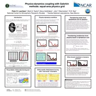
Physics-dynamics coupling with Galerkin methods: equal-area physics grid Peter H. Lauritzen1, Mark A. Taylor2, Steve Goldhaber1, Julio T. Bacmeister1, R.D. Nair1National Center for Atmospheric Research, Boulder 2 Sandia National Laboratories, New Mexico Introduction Consider a cubed-sphere tiling of the sphere with quadratic elements on each face. Inside each element there are 4x4 Gauss-Lobatto-Legendre (GLL) quadrature points: (Figure and caption from Nair et al., 2011) Assume a nodal basis set constructed using Lagrange polynomials hk(ξ), ξ=[-1,1]: where PN(ξ) is the Legendre polynomial of degree N and P’N(ξ) is the derivative of PN(ξ). With 4 GLL points there are 4 Lagrange basis functions (k=0,1,2,3). The solution U at time t inside element j is given by where Uj,k(t) is the known value at the kth GLL point. Note that the solution is expressed as a Lagrange interpolation polynomial. For simplicity we show only 1D examples; the 2D basis set can be constructed with a tensor product of the 1D basis functions: Physics-dynamics workflow Consider the continuous Galerkin finite-element method used in CAM-SE (NCAR’s Community Atmosphere Model – Spectral Elements). For simplicity consider a domain of 3 elements in 1D and let the initial condition be a “global” degree 3 polynomial (which can be represented exactly by the polynomial basis). This process is repeated for each Runga-Kutta step. Now the physical parameterization suite is called which, based on the atmospheric state at the GLL point values, computes tendencies at the quadrature points. Note that the solution is only C0 at element boundaries! This is typically where noise appears! Transferring state from dynamical core to physics Currently, the physics state is initialized from the values on the GLL points including edge points where the solution is only C0. We argue that parameterizations should be given a grid cell mean value for the atmospheric state rather than a (quadrature) point value. We define an equal-area physics grid in each element by dividing each element into equidistant control volumes and integrate the Lagrange basis functions over the finite-volumes (see the last figure in the box to the left). Note that using averages to transfer data to the physics grid moves fields away from boundary of elements where the solution is least smooth (in element interior the polynomials are C∞) Note that GLL points at element edges are shared between neighboring elements: The solution is advanced one Runga-Kutta step inside each element and then projected onto a C0 basis (GLL point values at element edges are averaged – blue curve above) Transferring tendencies from physics back to dynamical core While basis function integration provides a consistent and accurate approach for moving data from the dynamics to the physics, optimal techniques for moving in the other direction are less obvious. Current experiments are conducted using weighted averages. In the near term, we propose to reconstruct a polynomial, , that satisfies the mass-conservation constraint in all physics grid finite-volumes in element k where j =1,..,NC (NCis the number of physics grid finite-volumes in element k). This polynomial is then evaluated at the GLL points to provide physics tendencies to the dynamical core. Assume that there is only a physics update for the GLL point located at x=3 (purple point above). After physics has updated the atmospheric state at the GLL point(s), the polynomial is “reconstructed”. The point value is the local extrema and it is not representative of the average atmospheric state in a control volume around the GLL point • What should resolution of physics grid be? • NC = NP – 1: Physics grid has approximately the same number of degrees of freedom as the dynamics grid. • NC = NP + 1: This resolution would allow construction of basis to dynamics Lagrange basis. • For tracer advection on finite volume grid, matching the physics grid to the fvm grid allows tracer data to be passed between physics and dynamics with no interpolation (e.g., for CSLAM). • Much experimentation remains to optimize this process. Lagrange “reconstruction” for GLL point values, Uj,k(t) = {0,0,1,0} for k=0,..,3 Coarser? Finer? We argue that an equal-area finite-volume physics grid is more consistent. Initial results: Held-Suarez forcing with “real-world” mountains The problem: Grid-scale forcing and noise The spectral-element “reconstruction” is least smooth at the element boundaries where the C0 constraint is enforced. In climate simulations with CAM-SE, noise in topographically forced flow typically appears near element boundaries (see Figures below). • References • Nair, R.D., M.N. Levy and P.H. Lauritzen, 2011: Emerging numerical methods for atmospheric modeling Lecture Notes in Computational Science and Engineering, Springer, Vol. 80, pp.251-311. • Peter H. Lauritzen, Ramachandran D. Nair and Paul A. Ullrich, 2010: A conservative semi-Lagrangian multi-tracer transport scheme (CSLAM) on the cubed-sphere grid.J. Comput. Phys.: Vol. 229, Issue 5, pp. 1401–1424, DOI: 10.1016/j.jcp.2009.10.036. Figure: (left) 30 year average vertical pressure velocity for AMIP run using rough topography and no extra divergence damping. (right) Same as (left) but for precipitation rate. Contact PL: pel@ucar.eduURL: http://www.cgd.ucar.edu/cms/pel Information:SG: goldy@ucar.edu: URL:http://www.cgd.ucar.edu/staff/goldy