
Chapter 5 : Unit-root Testing and Cointegration Analysis
E N D
Presentation Transcript
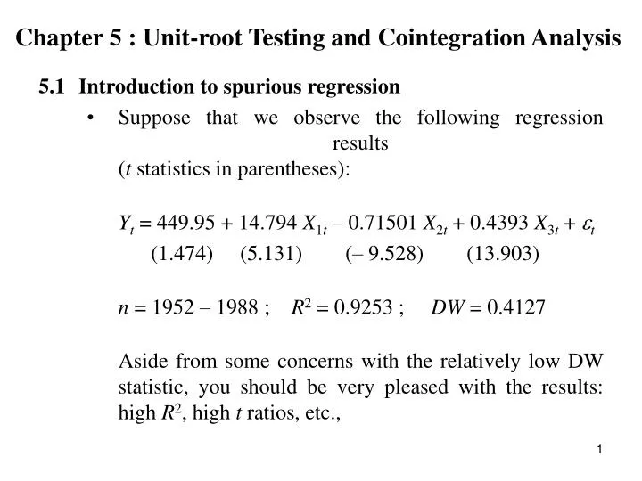
Chapter 5 : Unit-root Testing and Cointegration Analysis • 5.1 Introduction to spurious regression • Suppose that we observe the following regression results(t statistics in parentheses): Yt = 449.95 + 14.794 X1t – 0.71501 X2t + 0.4393 X3t + t (1.474) (5.131) (– 9.528) (13.903) n = 1952 – 1988 ; R2 = 0.9253 ; DW = 0.4127 Aside from some concerns with the relatively low DW statistic, you should be very pleased with the results: high R2, high t ratios, etc.,
But note : • Yt : Population in New Zealand; • X1t : Price level in China; • X2t : Money supply in China; • X3t : Per Capita Income in China.
Consider another amazing example • (from Hendry (1980): Econometrica): • Yt = 10.9 – 3.2 X1t + 0.39 X1t2 • (19.82) (13.91) (19.5) • n = 1945 – 1970 ; R2 = 0.982 ; DW = 0.1 • Notes : • Yt = Logarithms of C.P.I. in the U.K.; • X1t = cumulative rainfall in the U.K.
Obviously economic variables of China have no influence on the population of New Zealand. It would be equally absurd to conclude that the wet weather in Britain explains the rapid inflation experienced by the British economy. These are examples of “spurious regression”. Results occur because we are working with non-stationary data. • When using time series data, usual t-test; properties of R2 and OLS estimators, only typically applicable when variables are stationary. Signs of non-stationary are low DW but high R2.
5.2 Stationarity and Integration • Let yt be a time series variable. Then yt is stationary if the process which generates yt is invariant with respect to time: • If yt is stationary, then • (i) its mean E (yt); • (ii) its variance E((yt – E(yt))2); • (iii) covariance for any lag k; Cov(yt , yt-k) • are also invariant with respect to time.
Homogenous Non-stationary Process • Very few economic time series are stationary. But we can often “difference” a series to form a stationary process. Such a non-stationary series is called homogenous. • The order of homogeneity or order of integration is the number of times needed to difference the series to obtain a stationary series. Given this, we define a stationary series is defined as “integrated of order 0”, or I(0) • Specifically, we say • Ytis I(d) • That is, Ytis integrated of order d if • dYtis I(0), • where is the difference operator and d is the number of differences.
Example : Suppose Ytis a non-stationary homogenous series. Then if • Yt = Yt– Yt-1is stationary. That is, Yt ~ I(0). • Then Ytis integrated with order 1. • (b) Ytisalso non-stationary, but 2Yt ~ I(0), then Yt ~ I(2). • Generally, most economic time series are I(1) or I(2). Rarely are they I(0). • So what? Serious implications for regression analysis. Classical results, as discussed so far, assume data series are all stationary. Distribution of conventional statistics and estimators (for example, t ratios; regression coefficients; R2; F Ratio) for regression involving non-stationary variables are (typically) not at all like those derived under stationarity. So, it is very important to test for stationarity prior to proceeding with econometric analysis, if we want to avoid spurious results.
Now, suppose Yt ~ I(1), then • Ytcould follow a simple random walk process, That is, • Yt = Yt-1 + t • t is white noise. That is, tis an independently distributed random variable with zero mean and variance 2. In other words, Yt = Yt– Yt-1is a white noise process. Examples of random walk series are stock prices; future contracts; interest rates; exchange rates.
There are substantial differences between an I(0) series and an • I(1) series such as random walk. • (a) I(0) series has a finite mean and variance. There is a tendency for the the series to return to the mean. Conversely, a random walk will wander widely and will rarely return to an earlier value. Random walk has an infinite variance. • (b) Autocorrelation functions and Partial Autocorrelation Functions of I(0) and I(1) are different. • Autocorrelation for an I(0) series declines rapidly as lag(k) increases • The process gives low weight to events in the medium to distant past. That is, • I(0) series has a finite memory.
The Autocorrelation Function for an I(1) series are all near 1 in magnitude, even for large k. • The process has indefinitely long memory. • Similar pictures for the Partial Autocorrelation functions. For stationary series should decline to zero, while high magnitudes for non-stationary series.
Whether an economic time series is I(0) or I(d) , d 0, should be of serious concern to policy makers as it indicates whether the implication of a policy shock (tax change, welfare change etc.) are temporary or permanent. • For an I(0) series, any shocks are temporary. There is always a tendency for the series to move towards its finite. Constant mean. For an I(1) series, shocks have permanent effects.
General form of random walk • Random walk with drift • Yt = + Yt-1 + t • accounts for the non-zero mean in the differenced series. • (b) Random walk with drift and trend: • Yt = + Yt-1 + t +t • t = 1, 2, 3, … • That is, • Yt = + t+ t • So, general form of an I(1) series is • Yt = Yt-1 + +t +t (1)
Remarks: • (i) (1) is called a “unit root” model as it is a special case of a geneal AR(1) model : • Yt = Yt-1 + +t +t • with = 1 • If = 1, OLS estimation of (1) is inappropriate as data are non-stationary. Estimators and test statistics do not have the usual properties. • Removing drift and time trend does not help, as we are still left with the stochastic trend: • Yt = Yt-1 + t • Testing for a unit root ( = 1) was developed in the literature only in the last twenty years or so. A very popular test is the Dickey-Fuller (DF) (1981) test.
5.3 Testing for a unit root or the order of integration • Suppose • Yt = Ytor Yt-1 + +t +t 1 (a) • Then recall: • Random walk or unit root if = 1. Ytor detrended Ytareboth non- • stationary. OLS is not appropriate. • If 1 and > 0, then Ytgrowing because of positive deterministic • trend. • Detrended Ytis I(0). OLS is appropriate. • So, we test H0 : = 1. Unfortunately we cannot estimate (a) by OLS and do t-test using . OLS is biased towards zero if = 1 and so we could incorrectly reject H0 : = 1.
Dickey-Fuller (DF) test : • From (a) • Yt = Yt-1 + +t +t • Yt = ( – 1) Yt-1 + +t +t = Yt-1 + +t +t • If Ytis non-stationary, then = 1 and = 0 • If Ytis stationary, then < 1 and < 0 • So, testing = 1 is equivalent to testing • H0 : = 0 vs H1 : < 0 • If we do not reject H0, we believe Ytis I(1). • If we reject H0, we believe Ytis I(0).
To undertake the DF test: • Estimate Yt = Yt-1 + +t +tby OLS. Obtain • and the associated t-statistics. • Dickey and Fuller derived distribution of t-statistic: . • Test : < 0 compare t-stat with critical values from Table 1. • Remarks : • Dickey and Fuller derived large sample distribution of • t = . Note that is not Student’s t distributed. • Critical values for the test were calculated via Monte-Carlo simulation methods. Different authors report different critical values for the same sample size. We will use Dickey-Fuller’s tables.
Also, we need different critical values if we estimate (a) Yt = Yt-1 + t (b) Yt = + Yt-1 + t • However, it is usual to include a drift term , as = 0 implies the change series has zero mean which is not typically the case for economic data. • What about the linear time trend? No agreed strategy, but one approach (proposed by Dolado, Jenkinson and Sosvilla-Rivero (1990)) is to :
Estimate the following equation by OLS : • Yt = Yt-1 + + t +t • and obtain . • Test < 0 using “t-test”. Compare test statistic with critical values from Table 1. • If we reject H01, then we believe Yt is stationary. • If we cannot reject H01, then test • using a F type test. Compare calculated test statistic with Table 2. • (e) If we reject H02 test H01 again using the standard normal tables. If we reject H01, then Ytis stationary.
If cannot reject H02, then estimate • Yt = + Yt-1 + t • (That is, no trend term) • and test • H03 : = 0 vs H13 : < 0 • using “t-test” and compare with critical values in table 3. • If we reject H03 then we believe that the series is stationary. If we cannot reject H03, then the series is non-stationary. (We could also test but is usually significant with economic data).
Example 1 : • Suppose we estimate • Yt = + Yt-1 + t +t ; T = 50 • TestH01 : = 0 vs H11 : < 0using “t-test” • Suppose the calculated test statistic is –4.20. From Table 1, 10% critical value is – 3.18. So, we reject H0 and Yt is believed to be stationary. No further testing is required. • Suppose instead the calculated test statistic is –2.50. We cannot reject H0. So now test H02 : = = 0 vs H12 : < 0 ; 0 using a F type test. Suppose the calculated test statistic is 9.32. 10% critical value from Table 2 is 5.61. We reject H02 . • Then, re-test H01 : = 0 vs H11 : < 0using standard normal 10% critical value = – 1.2816. Clearly, –2.50 < –1.2816. We reject H01 and believe that Y1 is stationary.
For these test to be valid, we must have white noise residuals in the regression. • Frequently this is not the case. So it leads to the Augmented Dickey Fuller (ADF) test. • The aim is to add sufficient lags of Yt-j to ensure no autocorrelation in the residuals. But how to find P? • One way is to find the AF and PAF for the residuals from estimating (*) with P = 0, 1, 2 … until residuals are white noise. Then, having determined P, follow the testing strategy as given for DF test.
Testing for a unit root in the New Zealand population series using the Dickey-Fuller test • In this example, our aim is to determine the order of integration for the New Zealand population, over 1890-1991. The series in levels is depicted below – it is clearly non-stationary – at least in its mean. POP is also graphed – it is difficult to “guess” whether POP is stationary – its mean could well be, but the mean is clearly non-zero, suggesting that the D.F. models will require a drift term. There may well also be a positive trend but this is extremely difficult to ascertain from the graph.
We now turn our attention to formally testing, using the DF test, weather POP has a unit root – i.e., is the series stationary. Recall that the general model under test is : • POPt = POPt-1 + + t +t (1) • where, in particular, it is assumed that the disturbance is white noise. Recall from our earlier discussion that we first estimate (1) by OLS and test • H0 : = 0 vs H1 : < 0 (2) • using the “t-test” and the critical value from Table 1. The SAS commands and output follow:
data nzpop; input pop; t =_n_; lpop-lag(pop); dpop=pop-lpop; proc reg; model dpop=lpop t; run;
The appropriate t-stat is – 1.860. From Table 1, the 10% critical value for 100 observations (we have 101 here) is 1 3.17. Clearly, as expected, we cannot reject H0. Given this we now need to test: • H0 : = = 0 vs H1 : < 0, 0 (3) • using the “F-test”. This is usually undertaken using the “Lagrange Multiplier” or “Likelihood Ratio” tests.
The calculated test statistic is 6.695. From Table 2 the 10% significance level critical value is 5.47 (n = 100). So we reject H0 , and believe that the trend is significant. The procedure is to now re-test hypothesis (1) using the standard normal tables – at the 10% level and the critical value is –1.2816; –1.6449 at the 5% level, and –2.3263 at the 1% level. Our test statistic is –1.85988, so we reject H0 at the 5% level but not at the 1% level. Given this I would err on the conservative side and proceed as if we cannot reject H0 – that is, proceed as if POP is non-stationary and at least I(1).
Why at least I(1)? We have merely rejected that the series is stationary, it could be I(1) or I(2) etc. Our next step is to rerun the experiment using second difference, that is, estimate : • 2 POPt = POPt-1 + + t +t (4) • Let POPt = DPOP then we can write (4) as : • DPOPt = POPt-1 + + t +t (5) • Which is exactly the same form as (1) except in terms of DPOP. So, our interest now lies in whether = 0 in (5). If we cannot reject that = 0 then we believe that DPOP is I(1), i.e., POP is I(2). Conversely, if we reject the hypothesis that = 0, then we believe that DPOP is I(0), i.e., POP is I(1). If this occurs and given our previous result that POP is not I(0) then POP must be I(1).
Following are the SAS commands and output for estimating (4), or equivalently (5).data nzpop2;set nzpop2;1dpop=lag(dpop);d2pop=dpop-1dpop;proc reg;model d2pop=1dpop t;run;Model: MODEL1Dependent Variable: D2POP
The t-stat for the hypothesis of H0 : = 0 vs. H1 : < 0 is –3.966. From table 1, the 10% critical value is–3.17 (n = 100). We reject H0 – DPOP is I(0), so POP is I(1). We identify that the order of integration for POP is 1. Note that most economic time series are I(1) or I(2) – if a series is I(2) then we would accept H0 : I(2) vs. H1 : I(1) and so we take another difference and test H0 : I(3) vs. H1 : I(2), and so until we believe that H1 is appropriate.
Testing for a unit root in a New Zealand population series using the Augmented Dickey-Fuller test • We first need to determine the order of augmentation (if any) that is required to ensure that the residuals from the integrating regression are (approximately) white noise. That is, what is the value of p in • Below are the commands and outputs for determining p. data nzpop; infile ‘c:\teaching\ar3316\nzpop.dat’; input pop; t=_n_; lpop=lag(pop); dpop=pop-lopo; proc reg; model dpop=lpop t; output out=out1 r=e; run; proc arima data = out1; identify var=e nlag=10; run;
Are the residuals from this regression white noise? If so, then p = 0; that is the degree of augmentation is zero and the DF test is appropriate. If not, then the DF test is inappropriate and we do need to augment the integrating regression • Clearly, there is significant autocorrelations at k = 1 and k = 2 – the residuals are not approximately white noise, and the DF test is not appropriate. We now ask whether the residuals from the integrating regression with p = 1 are uncorrelated. data nzpop2; set nzpop; ldpop=lag(dpop); proc reg; model dpop=lpop t ldpop; output out=out2 r=e; proc arima data = out2; identify var=e nlag=10; run;
Of course, we can formally test whether any of these autocorrelations are significantly different from zero using a t-test, but we’ll simply “eyeball” the functions and see if there are any “large” spikes. I would believe not. This suggests that we can obtain (approximately) white noise residuals by setting p = 1. That is, we estimate, POPt= POPt-1 + + t + 1POPt-1 + t (1) • and using this model to test for stationarity of the series. We now proceed to do this following exactly the same strategy as we discussed for the DF test but applied to model (1) rather than to the DF integrating regression which assumes that p = 0. Fortunately, the critical values for the tests do not change as p changes. • We first test H0 : = 0 vs. H1 : < 0 • using the estimated t-stat on . From our printout this is −1.769. The 10% critical value from Table 1 of your handout with n = 100 is −3.17 – we cannot reject H0. We then proceed to test whether or not the trend term is significant : H0 : = = 0 vs. H1 : < 0; ≠ 0
So, the F stat is 1.966. From Table 2, the 10% critical value is 5.47 (n=100) – we cannot reject H0. That is, we cannot reject the trend is insignificant. Note that this is not the conclusion that we reached when we incorrectly used the DF test. So we now estimate, • (2) • determing p in the same way before. The commands and output for this follows:
Proc reg data=nzpop;model dpop=lpop;output out=out3 r=e;proc arima data=out3;identify var=e nlag=10;run;Model: MODEL1Dependent Variable: DPOP
Clearly, some significant autocorrelations. So, consider p=1,data nzpop3;set nzpop2;one=1;proc reg;model dpop=lpop ldpop one/noint;/output out=out4 r=e;proc arima data=out4;identify var=e nlag=10;Model: MODEL1NOTE: No intercept in model. R-square is redefined.Dependent Variable: DPOP
This looks reasonable – so we’ll proceed using p=1. We now test H0 : = 0 vs H1 : < 0 using the t-stat from this model with p=1. From the above printout this is 0.5541 – it is positive and so we know automatically that we cannot reject H0 . Following our strategy, given this result, we now need to test: H0 : = = 0 vs. H1 : H0not true
Test lpop=0, one=0;Dependent Variable: DPOPTest: Numerator: 808.8862 DF: 2 F value: 5.7076 Denominator: 141.7212 DF: 97 Prob>F: 0.0045 • We find the F statistic to be 5.708. the 10% critical value is 3.86 (from Table 4). So we reject H0 and believe that there is a significant drift term. We now need to re-test H0 : = 0 vs. H1 : < 0 using the standard normal critical value. Again, we know that these critical values are negative, and our t stat is 0.5541 – so we cannot reject H0 : POP is not I(0) and could be I(1). • We can continue this process and test I(1) vs. I(2) etc., and will eventually conclude that POP is I(1).
Integration results suggest that we should model non-stationary series when they are appropriately differenced. This is valid except when the variables of interest are non-stationary (integrated of the same order) and cointegrated. Then it is legitimite to estimate an economic model using undifferenced data. What do we mean by variables being cointegrated? We will only consider the two variable case. Consider a pair of variables xt and yt, each of which is I(d). The linear combination of xt and yt zt = yt – bxt (1) is also I(d). However, if there exists a constant b such that zt is I(0), then xt and yt are cointegrated. b iscalled “cointegrating parameter”. For the two variable case b is unique.