Download
1 / 30
320 likes | 482 Views
November 16, 2010. ECE 1001 - Introduction to Control Systems -. Jiann-Shiou Yang Department of Electrical & Computer Engineering University of Minnesota Duluth, MN 55812. Outline. Control Courses and Mathematical Foundations Introduction to Control Systems

E N D
November 16, 2010 ECE 1001 - Introduction to Control Systems - Jiann-Shiou Yang Department of Electrical & Computer Engineering University of Minnesota Duluth, MN 55812
Outline • Control Courses and Mathematical Foundations • Introduction to Control Systems ► Examples of Control System Applications ► What is a Control System? ► What is Feedback and What are its Effects? • Software (Matlab, Simulink, Toolboxes)
Systems & Control Courses ECE 2111 (Linear Systems & Signal Analysis) ECE 2006 (Electrical Circuit Analysis) Required ECE 3151 (Control Systems) ECE 5151 (Digital Control System Design) Elective ECE 8151 (Linear Systems & Optimal Control)
Mathematical Foundations • Vectors and Matrices† • Differential and Difference Equations† • Laplace Transform†‡ • Z-Transform‡ ____________________________________________ † Topics covered in Math 3280 (Differential Equations with Linear Algebra) ‡ Topic covered in ECE 2111 (Linear Systems and Signal Analysis)
More Advanced Control Study (for Graduate Control Courses) • Partial Differential Equations • Differential Geometry • Real Analysis • Functional Analysis • Abstract Algebra
Examples of Control Applications • Aircraft autopilot • Disk drive read-write head positioning system • Robot arm control system • Automobile cruise control system • etc.
What is a Control System? • A control system is an interconnection of components forming a system configuration to provide a desired system response.
Basic Control System Components • Plant (or Process) • - The portion of the system to be controlled - Process Process Output Input
Actuator • An actuator is a device that provides the motive power to the process (i.e., a device that causes the process to provide the output). • Sensor • Controller
Open-Loop Control Systems An open-loop control system utilizes an actuating device to control the process directly without using feedback. Input Actuating Device Process Output
Property: The system outputs have no effect upon the signals entering the process. That is, the control inputs are not influenced by the process outputs.
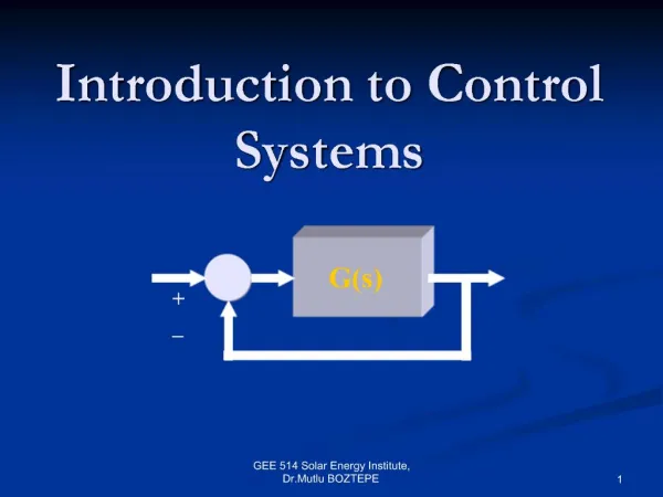
Closed Loop (Feedback) Control Systems A closed-loop control system uses a measurement of the output and feedback of this signal to compare it with the desired input (i.e., reference or command).
Comparison Comparison Controller Plant Output Desired Output Response Measurement Closed-loop: General Form
Example (Ref: Dorf and Bishop, Modern Control Systems, 12/e, Prentice Hall, 2011) Turntable Speed Control(Open-loop vs. Closed-loop) Many modern devices use a turntable to rotate a disk at a constant speed. For example, a computer disk drive and a CD player all require a constant speed of rotation in spite of motor wear and variation and other component changes. For the turntable speed control, the goal is to design a controller that will ensure that the actual speed of rotation is within a specified percentage of the desired speed despite all possible uncertainties.
Speed Turntable Adjustable Battery DCAmplifier DC motor Speed setting (a) Control Device Process Actuator Actual speed DC motor Amplifier Turntable Desired speed (voltage) (b) Turntable speed control: open-loop
Speed Turntable Adjustable battery DCAmplifier DC motor + _ Speed setting Tachometer (a) Error Actual speed Control Device Actuator Process + _ Amplifier Turntable DC motor Sensor Tachometer Measured speed (voltage) (b) Turntable speed control: closed-loop
Effects of Feedback on Sensitivity For the open-loop system shown below, if K2 is halved, then the system gain is also halved (i.e., the overall system gain reduces to 50% of its original gain) K1 K2 C R C = Gain = K1K2 R Controller Plant ‡ Note that for simplicity, we assume that K1 and K2 are constant. In general, they are frequency dependent.
Considerthe closed-loop system shown below: R-C K1(R-C) K1K2(R-C) R K1 K2 C + - K1K2(R-C) = C C K1K2 = R 1+K1K2 • Assume that K1K2 = 1 • If K2 is halved, then the overall system gain reduces to 67% of the • original gain. • Assume that K1K2 = 9 • If K2 is halved, then the overall system gain becomes 91% of the • original gain.
Conclusion • The sensitivity is reduced as the loop gain (i.e., • K1K2) is increased. Obvious advantage of using feedback
Effect of Feedback on Sensitivity (Cont’d) • -- Sensitivity to Plant Parameter Variations and • Model Uncertainty -- Controller Plant Gc G C R + - H Sensor
Closed-loop transfer function: C GCG T = = R 1+GCGH If GcGH >> 1 C GcG 1 T = ~ ≈ = R GcGH H
Effect of Feedback on Sensitivity (Cont’d) • If the loop gain GcGH >> 1, C/R depends almost entirely on the feedback H alone, and is virtually independent of the plant G and other elements in the forward path and of the variations of their parameters. • The sensitivity of the system performance to the elements in the forward path reduces as the loop gain is increased.
Effect of Feedback on External Disturbance D (disturbance) (command input) + + R C Gc G1 G2 + - (output) controller plant H sensor C G2 C GcG1G2 = = D 1+GcG1G2H R 1+GcG1G2H
For loop gain GcG1G2 >> 1, C 1 C 1 ≈ ≈ R D GcG1H H • If the loop gain GcG1G2 >> 1, then feedback reduces the effect of disturbance D on C if GcG1H >> 1 (i.e., the high gain is in the feedback path between C and D). • To ensure a good response to input R as well, the location of the high gain should be further restricted to GcG1, between the points where R and D enter the loop. • The sensitivity to disturbances reduces as this gain is increased.
Motivations for Feedback • The main reasons of using feedback are the following: • Reducing the sensitivity of the performance to parameter variations of the plant and imperfections of the plant model used for design • Reducing the effects of external disturbances and sensor noises • Feedback can also • Improve transient response characteristics • Reduce steady-state error
MATLAB (MATrix LABoratory) • Matlab is a software package developed by Mathworks for high performance numerical computation and visualization. It has been widely adopted in the academic community. • More than 3,500 universities around the world use MathWorks products for teaching and research in a broad range of technical disciplines (http://www.mathworks.com) • Matlab provides an interactive environment with hundreds of built-in functions for technical computation, graphics, and animation. • Matlab also provides easy extensibility with its own high level programming language.
Toolboxes • Toolboxes are libraries of Matlab functions that customize Matlab for solving particular classes of problems. • Toolboxes are open and extensible; you can view algorithms and add your own. • Toolboxes: control systems, communications, signal processing, robust control, neural network, image processing, optimization, wavelet, system identification, etc.
SIMULINK • Simulink is an extension to Matlab that allows engineers to rapidly and accurately build computer models of dynamical systems, using block diagram notation. • Simulink is a software package for use with Matlab for modeling, simulating, and analyzing dynamical systems. Its graphical modeling environment uses familiar block diagrams, so systems illustrated in text can be easily implemented in Simulink. • The simulation is interactive, so you can change parameters and immediately see what happens. It supports linear and nonlinear systems, modeled in continuous time, sampled time, or a hybrid of the two.
Mathworks Product Overview Simulink Product Family Application-Specific Products Matlab Product Family
Matlab and Simulink Tutorials are available in http://www.mathworks.com/academia/