Download

1 / 23
230 likes | 253 Views
This paper explores the use of maps to represent electron cloud (EC) density and its evolution in bunch-to-bunch interactions. The motivation is to minimize the detrimental effects of EC on beam instabilities, pressure rises, and heat load limits. The study includes phase transitions and the exploration of parameter space at RHIC.

E N D
Use of Maps for exploration of Electron Cloud parameter space Ubaldo Iriso and Steve Peggs M. Blaskiewicz, A. Drees, W. Fischer, H.C. Hseuh, G. Rumolo, L. Smart, D. Trbojevic, S.Y. Zhang. ECLOUD’04 April 19-23 2004, Napa, CA
Outline 1) Motivation: the bunch to bunch evolution 2) Can the Electron Cloud be represented by maps? 2.1. The first N=N and N=0. 2.2. Examples for the RHIC case 3) N exploration of parameter space 4) Electron Cloud phase transitions at RHIC 5) Conclusion and outlook
1. Motivation: the bunch to bunch evolution After experimental observations at RHIC during Run-3*, the use of gaps along the bunch train is chosen to minimize the detrimental effects of Electron Cloud (EC): • If EC density does not produce beam instabilities, • If the flux into the wall does not produce pressure rises above harmful limits, • If we are below heat load limit, then... who cares if EC is there? QUESTION: How do we evaluate the bunch pattern that minimizes EC density (->maximize luminosity? *BNL C-A/AP/118
1. Motivation: the bunch to bunch evolution • For a given surface and beam pipe dimensions and an initial electron cloud density ( ), what is the evolution after a bunch m passes by?
2. Can the EC be represented by maps? • For a given surface, for the EC build up the only thing changing between the bunch m and bunch m+1 is m and m+1 . That is… ! • Plot m+1 vs m : • Looks like a parabola that gets to the line y=x for saturation. • The EC build up using 3rd order fits look quite accurate… ; i > 1 and ai(N)!! Note: I don't show (m, m+1) corresponding to the first N=0 (first “no-bunch” in the abort gap). I will...
The first N=0 (first “no bunch” in the abort gap after a bunch train of M bunches with bunch charge N) is determined by another polynomial, and it is independent of N. This point in (rho_m+1, rho_m) is out of the N=0 line due to duration of space charge effects. 2. Can the EC be represented by maps? • Results for different N using CSEC (M. Blaskiewicz), and ECLOUD (F. Zimmermann). This is, results using different SEY parameterization: ECLOUD(Thanks G. Rumolo!) CSEC First N=0 curve First N=0 curve N=0 curve (decay) N=0 curve (decay) SEY from Furman & Pivi SEY from Cimino & Collins
N=N build up First N=0 N=0 decay (gap) • Much faster than following ns-to-ns using “typical” EC simulation codes (~1h vs ~1ms) 2. Can the EC be represented by maps? • Once we have ai (i=1,2,3) as a f(N), we just need an algorithm depending on Nm, being m the bunch number in the bunch train • Question: What’s the best way to distribute 68 bunches? Let’s see: We have quite a few possibilities… 110!/(110-68)!68! ~ 10^30
Example: the RHIC application • At RHIC, a given bunch pattern is determined by the triplet (Ks, Kb, Kg), where: • Ks: bucket spacing (multiple of 3 due to kicker limitations) • Kb: number of consecutive bunches with this bucket spacing • Kg: bunches not filled with this bucket spacing Unless otherwise noted, this is structure is repeated until the abort gap Example: (3,2,0)(6,4,0) – 3 bunches with 3 buckets spacing, followed by 4 bunches with 6 buckets spacing Some parameters to know about RHIC: Harmonic number, 360. Abort gap: 30 buckets. Bucket length: 35.6 ns. “Bunch harmonic number”:120. Abort gap, 10 bunches
N=N: Build up curve First N=N curve First N=0 curve N=0: Decay curve 2. Can the EC be represented by maps? evolution from CSEC for the BP (3,2,0)(6,4,0) The first N=N is needed!! Similarly to what happens with the first N=0, doesn’t jump from N=0 to N=N in only one bunch. When many successive bunches are filled, this “misalignment” is not significant.
Evaluating Maps for Electron Cloud (MEC) vs “usual” EC simulations codes (in this case, CSEC) gives now very good agreement. See next slides... 2. Can the EC be represented by maps? • Complete algorithm then, requires: N=N build up (N,N) First N=0 (0,N) N=0 gap (0,0) First N=N!! (N,0) (Nm , Nm-1 ) Note:MEC requires an initial 0 (seed).
2. Can the EC be represented by maps? Bunch pattern: (3,12,8) Bunch pattern:(3,2,0)(6,4,0) 1st turn 2nd turn 3rd turn 1st turn 2nd turn 3rd turn
2. Can the EC be represented by maps? Bunch pattern: (3,4,0)(6,8,0) Bunch pattern: (3,4,0)(6,8,0) FIRST N=N INCLUDED!! => Good agreement NO FIRST N=N INCLUDED!! => is overestimated
m+1 m m+1(m ) evolution for BP (3,2,0)(6,4,0) Nm Bunch Number 1 2 3 4 5 6 7 8 9 10 (N,0) (N,N) (N,N): linear coefficient a11 > 1 (0,N) (N,0): linear coefficient a10 >1 (< a11) (0,N): linear coefficient a01 < 1 (0,0) (0,0): linear coefficient a00 < 1 (< a01) (Nm, Nm-1)
3. N exploration of parameter space All the information for the EC build up can for a “regularly” distributed bunch train can be determined by ai coefficients. CSEC ECLOUD(Thanks G. Rumolo!) δmax=2.3
3. N exploration of parameter space: a map application Suppose the map: We have seen we need four sets of parameters, depending on , full bunch follows a full bunch a11, b11, c11 (N, N) , full bunch follows an empty one a10, b10, c10 (N, 0) , empty bunch follows a full one a01, b01, c01 (0 , 0) , empty bunch follows an empty one a00, b00, c00 (0 , N) If , remains always small enough, we can use linear approximation. After H possible bunches, having filled up to M bunches and i transitions (from 0 to N, and vice versa), the linear approximation says: , where F is:
3. N exploration of parameter space: a map application If F > 1; will increase (up to a saturated value, out of linear regime) If F < 1; the EC disappears. This factor is written as: For a given M, does not blow up if (a10·a01)/(a11·a00) < 1 Minimum F requires < 1 large values of i !! That is, maximum number of transitions, that is, the most sparse distribution of bunches minimizes EC. Current way to distribute bunches at RHIC to minimize EC
4. EC phase transitions at RHIC 50 Au 79+ x 109 25 Sudden pressure drop, while beam decays “adiabatically”. Do simulations reproduce this kind of “1st order phase transition”? 0 10-9 10-9 P (Torr) 10-10 10-11
4. EC phase transitions at RHIC • (P, N) diagram for the previous case:
4. EC phase transitions at RHIC 50 Not all places show 1st order phase transitions behavior. 2nd order types are also present for the same beam. Au 79+ x 109 25 0 10-9 IR10: 1st order P (Torr) 10-10 IR12: 2nd order 10-11
4. EC phase transitions at RHIC • (P, N) diagram for the previous case: IR10: 1st order behavior IR12: 2nd order behavior
4. EC phase transitions at RHIC Simulation results using CSEC for fine N: sat= (N-Nc) 2nd order behavior, analogy with Type II superconductors) Similar EC behaviors: -D. Schulte P(W/m) vs δmax (in ECLOUD’04) -M. Furman (LHC-Project Report 180) = 0.509 +/- 0.017 Nc = 7.398 +/- 0.005 Are the 1st order phase transitions reproducible with some code?
5. Conclusions… • From the EC simulation codes (CSEC), the multi-bunch EC build up for RHIC has been determined using a 3rd order polinomial map. Preliminary results from ECLOUD are promising. • A ‘memory’ of two bunches both for the decay as for the build-up is found. With this effect taken into account (“first N=0”, and “first N=N), agreement between MEC and CSEC is very good. • Given a machine limitation limit (due to heat load, pressure rise, instabilities…), MEC is useful for RHIC to find out the best way to live with EC by changing the bunch pattern • Using maps, exploration of (,N) is done, and standard maths are used to justify sparse distribution for bunches along a bunch train. • 1st order and 2nd order phase transitions are seen at RHIC, but only 2nd order phase transitions seems to be reproducible with the codes.
… and outlook • How do coefficients vary with SEY, R, etc follows. Can we find some few parameters to describe EC (sic). • Can we map EC from experimental data? • Does it work for *your* machine with *your* code? • Is it an artefact due to long RHIC bunch spacing? Can we go to shorter bunch spacings? B-factories? • Are the 1st order phase transitions reproducible with EC codes? … and acknowledgements… M. Blaskiewicz, A. Drees, W. Fischer, H.C. Hseuh, R. Lee, N. Luciano, G. Rumolo, L. Smart, R. Tomás, D. Trbojevic, L. Wang, S.Y. Zhang.