Download
1 / 30
300 likes | 315 Views
Explore the implications of discrete vs. continuous data, map data types, contouring, and spatial reasoning in GIS modeling. Learn about spatial statistics and the frontier of multimedia mapping. Discover various map types like base, derived, constraint, and final maps.

E N D
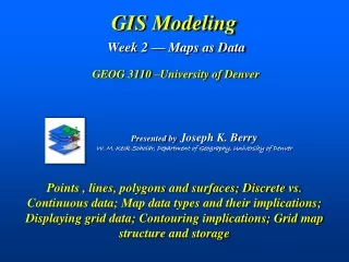
Presented byJoseph K. Berry W. M. Keck Scholar, Department of Geography, University of Denver GIS ModelingWeek 2 — Maps as Data GEOG 3110 –University of Denver Points , lines, polygons and surfaces; Discrete vs. Continuous data; Map data types and their implications; Displaying grid data; Contouring implications; Grid map structure and storage
Who We Are (Class Photo) <as of Thursday morning> Student Statements posted at… … Class Website Email_dialog/StudentStatements.htm#Student_statements
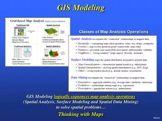
Now, Where Were We? GIS Modeling What GIS Is (and isn’t) Computer Mapping (70’s) - Spatial dB Management(80’s) - GIS Modeling (90’s) • Spatial Analysis— “contextual” relationships within and among mapped data (Reclassify, Overlay, Distance, Neighbors) From mapping to Spatial Reasoning… …that radically changes our Map Paradigm • Spatial Statistics — • “numerical” relationships within and among mapped data (Surface Modeling and Spatial Data Mining) …keeping in mind that the current frontier is focused on Multimedia Mapping (00’s) (Berry)
1 2 3 4 1) Base maps 2) Derived maps 6 3) Interpreted maps 4) Combined / Modeled maps 5) Constraint maps 5 6) Final map Campground Suitability Model Review (Logic) Prefer Gentle Slopes, Near Roads, Near Water, View of Water and Westerly Oriented …but can’t be too close to water or too steep Best Green Worst Red Constrained Black (Berry)
Solution set of maps are created by evaluating the model logic for the unique pattern of conditions at each geographic location …grid cell Campground Suitability Model Review (Solution) A sequencing of map analysis commands are applied to implement model logic—using a command script(Tutor25_Campground.scr) Best Green Worst Red Constrained Black (Berry)
Spatial Data vs.Spatial Information (digital slide show BB-BK) From GIS as a Toolboxenabling display and geo-query to a Sandboxfor developing, communicating, interacting and evaluating solutions to complex spatial problems— …from Where is Whatto So What, Why and What If Spatial Reasoning and Dialogue Tropical Resources Institute Yale University — 1988 Consultant Heaven Infusing Stakeholder Perspectives Compaq II Portable Computer Summagraphics Bit Pad Digitizer Consultant Hell (Berry)
Manual cartography utilizes points, lines and areas as the basic building blocks for characterizing geographic space Based on spatial objects (discrete) New map feature type based on grid cells (continuous) …traditionally all maps are composed of three fundamental map features—Points, Lines and Areas. The digital map provides additional dimensions of depth and time to extend the features to Surfaces, Volumes, hyper-Volumes and fuzzy-Features Basic Map Features (Berry)
Storing Points, Lines and Areas …how do you think Vector and Raster data structures store Surfaces, Volumes, hyper-Volumes and fuzzy-Features? (Berry)
…heresy!!! Spatial Resolution The concept of Scale (S= Map Distance /Ground Distance) …replaced by the concept of Resolution(Spatial, Mapping, Thematic and Temporal) does not exist in a GIS (Berry)
Minimum Mapping Resolution …replaced by the concept of Resolution(Spatial, Mapping, Thematic and Temporal) (Berry)
Thematic and Temporal Resolutions …replaced by the concept of Resolution(Spatial, Mapping, Thematic and Temporal) …so what is the difference between the concepts of PRECISIONand ACCURACY …and how do these concepts relate to the concept of RESOLUTION? (Berry)
Handheld GPS unit Accuracy describes the closeness of arrows to the bull’s-eye at the target center (actual/correct) High Accuracy but Low Precision Accuracy vs. Precision …the “target analogy” compares measurements to the pattern of arrows shot at a target High Precision but Low Accuracy Precision GPS unit Precision relates to the size of the cluster of arrows— grouped tightly together is considered precise Accuracy versus Precision The Wikipedia defines Accuracy as “the degree of veracity” (exactness) while Precision as “the degree of reproducibility” (repeatable) (Berry)
Interpreter A Interpreter B Interpreter C Vegetation Parcel Mapping Superimposed interpretation boundaries Accuracy = classification (What) Precision = delineation (Where) Photo Interpreter A Cottonwood Photo Interpreter C Cottonwood Photo Interpreter B Ponderosa Pine Classification versus Delineation (spatial perspective) Classification Accuracy (What) Delineation Precision (Where) (Berry)
Routing Criteria Most Preferred Least Preferred 1 2 3 4 5 6 7 8 9 RP & SA times 10 HD & RP times 10 HD & VE times 10 Environmentalists Engineers Homeowners Start Start Optimal Path Optimal Corridor Engineers Environmentalists Homeowners Average of the three cost surfaces Combined Solution Individual Solutions End End Model Accuracy/Precision (spatial modeling perspective) Calibrate Expert Opinion Housing Density Road Proximity Sensitive Areas Visual Exposure …cognitive mapping has no definitive right/wrong solution— Most Preferred Weight Stakeholder Values (Berry)
It is important to note that the map features in a vector-based mapping system identify discrete, irregular spatial objects with sharp abrupt boundaries. Raster data types —grid surfaces, raster imagesandpseudo grids— treat space in entirely different manner to portray spatially continuous data …in araster image (aka photo) the values stored at each map location identify its color (hue, saturation and brightness)– constrained integer value (0-255) …mapped data ready for map analysis and modeling • GIS Maps contain— • Points, lines, polygons • Grid surfaces • Raster images • Pseudo grids …in apseudo grideach grid element is treated as a separate polygon (square) with spatial and attribute tables defining the set of little polygons Raster Data Types Map Layer (Berry)
Basic Grid Data Structure A Grid Mapconsists of a matrix of numbers with a value indicating the characteristic /condition at each grid cell location Map Stack …forming a geo-registered set of Map Layers or “Map Stack” Lines Grid Map Layer Mesh Fill Analysis Frame TheAnalysis Frame provides consistent “parceling” needed for map analysis and extends discrete Point, Line and Areal features to continuous Map Surfaces Col 3, Row 22 Data listing for a Map Stack Drill-down Layer Mesh
Basic Grid Display Types Display Types… Lattice display forms a smooth wireframe Griddisplay forms chunky extruded grids …so how is a Contour Map generated? (vector representation of a surface) Contour line 1900 (See Example Applications, “Display Types” for more information) (Berry)
Thematic Display (Shading Manager) MapCalc Shading Manager… # Rangessets the number of intervals Equal Rangeshas the same range for each interval Equal Count has the same number of cells for each interval (See Example Applications, “Display Types” for more information) (Berry)
+/- 1Stdev Equal Count Equal Ranges User Defined (300 Step) Contouring Mapped Data (Continuous to Discrete) • Display the elevation surface as wireframe (Lattice) with filled floor contours • Set #Ranges to 7 and assign yellow as the inflection color • Redisplay the surface as Equal Count, Equal Ranges, StDev and User Defined …note the dramatic differences in the shape and position of the boundary lines of the discrete contour intervals So which discrete map of elevation surface is CORRECT? (Berry)
3D Togglechanges 2D and 3D display forms Display Form… Use Cellstoggles between Lattice and Grid display types Display Type… Data Typetoggles between Discrete and Continuous data types Data Type… Matching Data Types & Display Types/Forms (See Example Applications, “Data Types”, “Color Interval/Pallet”, “3D Display Options” and “Data Inspection and Charting” for related information) (Berry)
Numeric and Geographic Data Types …all digital maps are composed of organized sets of numbers— the Data Type determines what “map-ematical” processing can be done with the numbers on a map, or stack of map layers (Berry)
Homework Exercise #2 • Part 1 – Understanding Basic Concepts and Terms • Scale and Resolution. 1) Map Scale, 2) Spatial Resolution, 3) Thematic Resolution, 4) Minimum Mapping Resolution and 5) Temporal Resolution. • Data Types. 1) Nominal, 2) Ordinal, 3) Interval, 4) Ratio, 5) Binary, 6) Choropleth, 7) Isopleth data types (be sure to distinguish which data types are Numeric and which are Geographic) • Display Considerations. You will generate different map displays of the Slope and Districts map layers, then identify/comment on the Data Type, Display Type and Display Form used and discuss the effects/appearance of the different displays • Part 2 –Characterizing Geographic Space …Discrete versus Continuous • Thematic Mapping. You will use the Shading Manager to create different map displays while investigating the effects of Calculation Mode (Equal Ranges, Equal Count,+/- 1 Standard Deviation and User Defined), Number of Ranges and Color Ramp assignments. (Berry)
(Exercise #2, Part 3) • Create a slope map • Reclassify that map for slope classes • Create a flow map • Reclassify that map for flow classes • Combine the maps of slope classes and flow classes • …result is a map with a 2-digit code 1St digit = flow class 2nd digit = slope class Simple Erosion Model (Berry)
So Where Are You in GIS? “…of the Computer” “…of the Application” …changing our Map Paradigm General and Innovative Users– uses understanding of basic concepts, capabilities and considerations in developing new applications within their discipline “…of the Discipline” The “bookends” of this continuum are the current drivers of Geotechnology Data Provider– develops GIS data layers; good skills in GPS and remote sensing with strong skills in GIS data formats and geodetic referencing Systems Manager– develops and maintains spatial databases and connections within (LAN) and outside (Internet) the organization; CS and GIS balance Solutions Developer– develops GIS applications that link GIS to real-world problems; mostly GIS/CS with some disciplinary expertise Computer Programmer– develops GIS tools; mostly computer science with some courses in GIS GIS Specialist– uses discipline expertise and GIS knowledge for basic GIS applications and interacts with solution developers to address complex spatial problems (See Beyond Mapping III, Topic 4, “Where Is GIS Education”) (Berry)
V to R– burning the points, lines and areas into the grid (fat, thin and split) R to V– connecting grid centroids, sides and edges (line smoothing) Vector to/from Raster (direct calculation) (Berry)
V to R– uses a point file of cell centroids and converts polygon features that intersect Implied Grid with Centroids Centroid Point File Vector Map (polygons) The corresponding grid cell is assigned the value of the “point in polygon intersection” Polygons with Overlaid Points Raster Map Vector to Raster (centroid implied) …as the points fall Note: this technique is very sensitive to cell size (features smaller than cells) and complexity of boundary shape …but it is really fast (Berry)
Exporting MapCalc Data Layers ESRI GridASCII Format just for fun (you are having fun, right?)— Export the MapCalc Tutor25.rgs Elevation map layer in both ESRI GridASCIIformat and Surfer ASCIIformat …browse to an appropriate folder and Save exported file Surfer ASCII Format (Berry)
…open the ELEV.asc file in Notepad to see the data structure (stored as an Individual File) <export Elevation as ESRI_elevation.asc and open in NotePad> Map Data (Bottom portion) Origin is upper-left corner …values along the row, left to right in a block (25) General Information (“header” first 6 records) Each block contains all of the map values for a row …next row up …repeat for all rows (625 total) Grid-based Data Structures/Formats(Esri .asc) #Row #Col Longitude of LL corner Latitude of LL corner Cell size (in decimal degrees) No Data value (null) (Berry)
…open the ELEV.grd file in Notepad to see the data structure (stored as an Individual File) <export Elevation as Surfer_elevation.grd and open in NotePad> Map Data (Bottom portion) Origin is lower-left corner …values along the row, left to right in a block (25) General Information (“header” first 5 records) Each block contains all of the map values for a row …next row up …repeat for all rows (625 total) Grid-based Data Structures/Formats (Surfer .grd) File Type #Row #Col Lon/Lat LL and UR Min and Max Value (Berry)
…open the Tutor25.rgs in Notepad to see the data structure (stored as a Data Table) …open Tutor25.rgs in Notepad Map Data (Bottom portion) Origin is lower-left corner …values for all columns along the row, left to right (25) Each column contains all of the map values for a layer General and Map Legend Information (top portion) …next row up …repeat for all rows (625 total) Grid-based Data Structures/Formats (MapCalc .rgs) (Berry)

![Data Modeling [Comparison of data modeling techniques ]](https://cdn0.slideserve.com/205866/data-modeling-comparison-of-data-modeling-techniques-dt.jpg)