Download
1 / 21
210 likes | 496 Views
Creation of topographical maps and modeling of brain plasticity. Włodzisław Duch Department of Computer Methods Nicholas Copernicus University Toruń, Poland Google: W. Duch. Plan. Intro: topographical maps everywhere Somatosensory maps Theoretical models

E N D
Creation of topographical maps and modeling of brain plasticity. Włodzisław DuchDepartment of Computer MethodsNicholas Copernicus UniversityToruń, PolandGoogle: W. Duch
Plan • Intro: topographical maps everywhere • Somatosensory maps • Theoretical models • What is to be explained in visual map formation? • Assumptions and types of models • Summary and conclusions
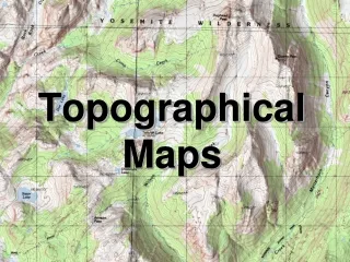
Topographical maps • Topographic representation of spatial patterns: key feature of visual and tactile data analysis; used also by motor and auditory system. • Serves locomotor navigation and object recognition. Tactile and motor maps: homunculus representation, cortex and cerebellum • Visual system - many maps of different type: • retinal projection on LGN of the thalamus; • retinotopic maps in V1 • SC multimodal maps …
Somatosensory maps • SI cortex: touch, pain, vibration, temperature. • Somatosensory and motor maps: Woolsey (1949), Penfield (1959), motor and sensory homunculus. • Some examples of homunculi: Note: representation of face is separate from the rest of the body. Molecular basis: ephrin-A5 ?
Model of self-organization SOMF, Self-Organized Feature Mapping, or Kohonen map. Simplest model of topographic self-organization via competitive Hebbian activity-dependent learning. Signal X activates most strongly a neuron with synapses W; they become more similar to X and also neurons in the vicinity of W become more similar to X. Receptive fields of neurons that are close on the 2D map are close in the input space. Update equation:
Global Somatosensory Map Data: 3D coordinates of 40 body areas, density of points prop. to inverse resolution, 600 pointsTest points: interpolation, 160 labeled points SOM map: long and narrow, 20x5, hexagonal neighborhoods. Why head/neck between legs/hands, but face outside? 5. thumb, 6. 2nd finger 7. 13. face 4. leg, 9. foot, 10. toes3rd finger 8. 4th finger 11. back, 12. chest 1. forearm 2. upper arm 3. shoulder
Theoretical accounts • Only a few papers on somatosensory or motor maps; no papers on global features of homunculus maps. • Few papers on Superior Colliculus maps (saccade generation). • Orientation and ocular dominance maps in V1 studied most frequently. • Usually simulations of neural dynamics at mesoscopic level. • Few papers based on neural field approach, spin systems and analytical considerations. • Erwin, E., Obermayer, K., and Schulten, K.J. (1995). Models of orientation and ocular dominance columns in the visual cortex: A critical comparison. Neural Computation, 7(3):425-468 • Swindale, N.V. (1996). The development of topography in the visual cortex: A review of models. Network 7(2):161-247.
Stability of maps Maps were considered static in adult animals, but: Brown, T.G, Sherrington, C.S (1912) On the instability of a cortical point. In 'critical' period of development (6 days in rats): Visual deprivation change physiological (Wiesel and Hubel, 1963, 1970) and anatomical monocular organization of afferents into visual cortex. Changes in the thalamocortical projections due to damage to peripheral nerves. Somatosensory deprivation in young animals (destroying whiskers in a neonatal rat) leads to changes in topography of the whisker representations (barrel field), responding to stimulation of other body regions (Waite and Taylor, 1978).
Plasticity of maps • Evidence for plasticity in adult animals from: • limb amputations or nerve lesions, from rodents to primates • Review: Gilbert, C.D. (1993) Rapid dynamic changes in adult cerebral cortex. Curr. Opin. Neurobiol. 3: 100-103 • Reorganization is a common feature of topographic sensory cortical maps. • Demonstrated in visual, somatosensory and auditory cortex. • Plasticity extends to higher cortical areas. • Many processes contribute to functional reorganization, different temporally and physiological dynamics. • Changes in receptive field size and location - minutes after lesions; reorganization of other systems - days to weeks (Kossut, 1988). • Mechanisms probably common to all cortical maps, may play a role in normal functioning, activity-dependent mechanisms are critical for maintenance of topographic maps.
Mechanisms of plasticity • Loss of input, changes in intensity or pattern of the afferent drive to the region at the physiological level leads to: • Fast: unmasking of existing connections which were normally ineffective, ex. unmasking via release of inhibition. Thalamic afferents may reach 10 columns; blocking cortical inhibition increases receptive fields. • Medium: activity dependence within intracortical circuits, with Hebbian preference to the most active inputs, competition for synaptic sites coupled with somatotopic continuity and overlap. Strengthening of polysynaptic pathways. • Longer time scales: sprouting of terminals from new sources. Demonstrated in the spinal cord.
Experimental facts • Optical recordings from large surfaces of macaque visual systems. • High resolution but only superficial layers. • Elements of orientation selectivity patterns: • Linear zones with iso-orientation contours, 0.5-1 mm • Singularities - 180 degree change, clockwise or anticlockwise. • Saddle points - almost constant orientation. • Fractures - rapid change across a line. • Characterize various features of such maps in statistical way. • Find theoretical model at mesoscopic level, matching the level of experimental observations.
Orientation + dominance • Contour plot: black contours - bands of eye dominance; gray lines - isoorientation. • Singularities usually near centers of ocular dominance bands. • Saddle points also near centers. • Local orthogonality and global orthogonality. • Global disorder - autocorrelation function. • Correlation between orientation and eye dominance. • Differences between preferred orientations and the direction of gradient of preferred orientations. • Distribution of orientation specificities. • ….
Theoretical assumptions • Large 2-D grid of elements representing neural assemblies, reacting to signals in their receptive field (spatial filters). • Feature vector representation: receptive field position, dominance, orientation angle, orientation preference, color information … • Weight vector representation: synaptic strength, high-dimensional. • 3 important principles: • Continuity - nearby columns react to stimuli with similar features - choice of similarity affects patterns. • Diversity - whole feature space should be covered. • Global disorder • Models may look quite different but are based on similar principles.
Theoretical models • Models proposed so far belong to 5 categories: • Structural models, assuming specific projections due to thalamic organization. • Spectral Models, filters in Fourier space. • Correlation-based learning, linear intra-cortical interactions with Hebbian learning. • Competitive Hebbian models, non-linear lateral interactions. • Mixed models and untypical models.
Structural models • Structural models, assuming specific projections due to thalamic organization. • The icecube model of Hubel and Wisel (1974) • The pinwheel model of Breitenberg and Breitenberg (1979) Extensions: Götz 1987 Baxter and Dow 1989 Problems with: global disorder, fractures. In a) no singularities or saddlepoints, in b) wrong singularities.
Spectral models Spectral Models, filters in Fourier space. Swindale 1980-92; Rojer and Schwartz 1990; Niebur and Wörgötter 1993 One-step models, very few parameters: n(r), white-noise patterns, Gaussian numbers around 0, as input h(r), representation of a band-pass filter H(n) Ocular dominance z(r) obtained from convolution of n(r) and h(r) Orientation map: u = grad z(r); Orientation preference q=||u|| Rojer, Swindale: wrong predictions of correlations between orientation preferences and cortical locations, since all closed integrals vanish. Iterative models (Swindale map1 and map2): F(t+1) = F(t) + a (F(t)*h(r)) f(F(t)); 0<a<1 f(F(t)) = (1-||F(t)||) introduces correlation of select/dominance
Correlation-based models Hebbian linear models. Miller, Keller, Stryker 1989 high-dimensional model: x - retinal location, r - cortical. For each eye separately Fi(t) ={Wi(t)} Fi(t+1) = Fi(t) + aA(r,x) [I(r,r’)*C0(x,x’)*Fi(t)+I(r,r’)*C1(x,x’)*F1-i(t)]; where A(r,x) describes location and size of receptive fields; I(r,r’) is intracortical interaction of the Mexican hat type; C0 is a correlation functions for the same eye, C1 for different eyes; Non-linearities may be added by normalization of weight vectors or limiting their range. Newer models (Miller et al 1990-2000): separate populations of ON and OFF-centered cells in LGN, more compelx reccurent models.
Competitive Hebbian models Low dimensional (SOM-l):at least (r, q sin(2f), q cos(2f), z(r)), i.e. position r(x,y), degree of orientation preference q, orientation angle f, dominance z. Ft+1(r) = Ft(r) + a H(r,r’)[Vt+1-Fi(t)]; Stimulus V is chosen at random, the neighborhood H(r,r’) is Gaussian around the winner r’ using Euclidean distance. High-dimensional (SOM-h): Ft+1(r) = {Wi(r)} normalized weights, i.e. Ft+1(r) = (Ft(r) + a H(r,r’)Vt+1)/||(Ft(r) + a H(r,r’)Vt+1)|| and correlation distance function d(V,W)=1-VW
Elastic Net Elastic net (Durbin and Wilshaw 1987) Similar to SOM, adds “elastic” term Ft+1(r) = Ft(r) + a H(r,r’)[Vt+1-Fi(t)] + bS [Ft(r) -Ft(r’)] ; with summation over r’ units nearest to r. Competitive Hebbian models simulate correctly strabismus and development of maps for biased or restricted patterns. Allow for joint pattern development of ocular dominance and orientation. Linear zone are perhaps less prominent as they should be, but with the present experimental data it is hard to quantify.
Summary of results • Linear zones: perhaps less prominent in correlation-based models and SOM-h. • Singularities: arise spontaneously in most models but missing or wrong in some structural models; saddle points wrong only in Icecube model. • Fractures: correct in most models; Miller and Linsker models predict discontinuities but higher map resolutions are needed to resolve this. • Global disorder: missing only from structural models. • Orthogonality: local appears in most models but may be too strong in SOM-l and EN; global may be a separate property, addressed only by Sindale’s model • Power spectrum: wrong in some models, low-pass instead of band-pass filters. • Distribution of feature specificities: correct in models that include them. • Anisotropies, monocular deprivation: easy to get. • Orientation deprivation, bias, joint development of occularity and orientation, correlations of higher orientation specificity with occularity: only in competitive Hebbian?
Conclusions • Structural models (Hubel, Wisel, Breitenberg) do not agree with experimental data. • Competitive Hebbian approaches have qualitative properties that agree with almost all experimental data. • More precise data are needed to eliminate other models. • Orientation selectivity is probably activity driven but … models using recurrent lateral connections may explain it using only intra-cortical dynamics; including contrast-invariance of orientation tuning, development of the orientation tuning may help to answer to what degree this mechanism is sufficient. Interplay between theory/experiment is essential to understanding topographical maps.