Download
1 / 14
140 likes | 221 Views
Extrasolar planet detection: a view from the trenches. Alex Wolszczan (Penn State) 01/23/06 Collaborators: A. Niedzielski (TCfA) M. Konacki (Caltech). Ways to find them…. Methods that actually work …. Radial velocity. Pulse timing. Microlensing. Transit photometry. Some examples….

E N D
Extrasolar planet detection: a view from the trenches Alex Wolszczan (Penn State) 01/23/06 Collaborators: A. Niedzielski (TCfA) M. Konacki (Caltech)
Methods that actually work … Radial velocity Pulse timing Microlensing Transit photometry
Some examples… Neptune-mass planet The transit classic: HD209458 Microlensing planet A “super-comet” around PSR B1257+12?
Orbits from Vr measurements • Observations are given in the form of a time series, Vr(i), at epochs t(i), i = 1,…,n • A transition from t(i) to (i) is accomplished in two steps: Equation for eccentric anomaly, E • From the fit (least squares, etc.), one determines parameters K, e, , T, P
…and from pulsar timing • In phase-connected timing, one models pulse phase in terms of spin frequency and its derivatives and tries to keep pulse count starting at t0 • A predicted time-of-arrival (TOA) of a pulse at the Solar System barycenter depends on a number of factors:
Determining binary orbits… • Collect data: measure Vr’s, TOA’s, P’s • Estimate orbital period, Pb (see below) • Use Vr’s to estimate a1sini, e, T0, Pb, (use P’s to obtain an “incoherent orbital solution”) • Use TOA’s to derive a “phase-connected” orbital solution
Figuring out the orbital period… • Go Lomb-Scargle! If in doubt, try this procedure (borrowed from Joe Taylor): • Get the best and most complete time series of your observable (the hardest part) • Define the shortest reasonable Pb for your data set • Compute orbital phases, I = mod(ti/Pb,1.0) • Sort (Pi, ti, I) in order of increasing • Compute s2 = ∑(Pj-Pj-1)2 ignoring terms for which j- j-1> 0.1 • Increment Pb = [1/Pb-0.1/(tmax-tmin)]-1 • Repeat these steps until an “acceptable” Pb has been reached • Choose Pb for the smallest value of s2
… and the latest puzzle to play with • Timing (TOA) residuals at 430 MHz show a 3.7-yr periodicity with a ~10 µs amplitude • At 1400 MHz, this periodicity has become evident in late 2003, with a ~2 µs amplitude • Two-frequency timing can be used to calculate line-of-sight electron column density (DM) variations, using the cold plasma dispersion law. The data show a typical long-term, interstellar trend in DM, with the superimposed low-amplitude variations • By definition, these variations perfectly correlate with the timing residual variations in (a) Because a dispersive delay scales as 2, the observed periodic TOA variations are most likely a superposition of a variable propagation delay and the effect of a Keplerian motion of a very low-mass body
One of the promising candidates… • Periods from time domain search: 118, 355 days • Periods from periodogram: 120, 400 days • Periods from simplex search: 118, 340, also 450 days
…and the best orbital solutions • P~340 (e~0.35) appears to be best (lowest rms residual, 2 ~ 1) • This case will probably be resolved in the next 2 months, after >2 years of observations
Summary… • Given: a time series of your observable • Sought: a stable orbital solution to get orbital parameters and planet characteristics • Question: astrophysical viability of the model (e.g. stellar activity, neutron star seismology, fake transit events by background stars) • Future: new challenges with the advent of high-precision astrometry from ground and space and planet imaging in more distant future