Unified Retrieval of Radiatively Consistent Cloud, Precipitation, and Aerosol Profiles

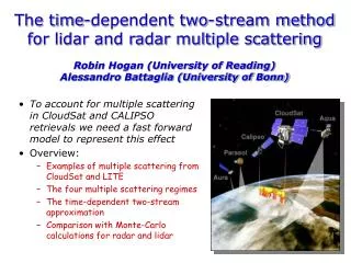
Grand Unified AlgorithmsHow to retrieve radiatively consistent profiles of clouds, precipitation and aerosol from radar, lidar and radiometers Robin Hogan, University of Reading Thanks to Julien Delanoe, Nicola Pounder, Nicky Chalmers, Howard Barker …and evaluating models

Spaceborne radar, lidar and radiometers The A-Train • NASA • 700-km orbit • CloudSat 94-GHz radar (launch 2006) • Calipso 532/1064-nm depol. lidar • MODIS multi-wavelength radiometer • CERES broad-band radiometer • AMSR-E microwave radiometer EarthCare • EarthCARE: launch 2012 • ESA+JAXA • 400-km orbit: more sensitive • 94-GHz Doppler radar • 355-nm HSRL/depol. lidar • Multispectral imager • Broad-band radiometer • Heart-warming name 2013 2015 2016 2017 2018 2019 2014

What do CloudSat and Calipso see? • Radar: ~D6, detects whole profile, surface echo provides integral constraint • Lidar: ~D2, more sensitive to thin cirrus and liquid but attenuated • Radar-lidar ratio provides size D Cloudsat radar CALIPSO lidar Insects Aerosol Rain Supercooled liquid cloud Warm liquid cloud Ice and supercooled liquid Ice Clear No ice/rain but possibly liquid Ground Target classification Delanoe and Hogan (2008, 2010)

How do we evaluate models? • New approach • Forward-model observations and evaluate in obs. space • IceSatlidar: Chepfer et al. (2007), Wilkinson et al. (2008) • CloudSat: Bodas et al. (2008) • CloudSat & Calipso: IPCC/COSP • Much easier! • Avoids contamination by a-priori information • Avoids competition between retrievals • Traditional approach • Compare retrieved cloud products to model variables • But these are the variables we want to know! • Simple forward modeling can get right answer for wrong reasons, e.g. right Z with wrong IWC and re • Can extract “hidden” info, e.g. re from radar-lidar synergy • Can provide radiative verification of each retrieved profile • But certainly more difficult!

Overview • Justification for and design of unified algorithm • Ice clouds • Evaluation against CERES • Evaluation of ECMWF and Met Office models • Liquid clouds • Fast multiple scattering model for exploitation of lidar signal • Extinction profile from multiple field-of-view lidar • Can we estimate liquid cloud base from the Calipso lidar? • First results from unified algorithm applied to A-Train • Simultaneous ice, liquid and rain retrievals • Outlook • 3D radiatively consistent scene retrieval

“Grand Unified Algorithm” • Combine all measurements available (radar, lidar, radiometers) • Forms the observation vector y • Retrieve cloud, precipitation and aerosol properties simultaneously • Ensures integral measurements can be used when affected by more than one species (e.g. radiances affected by ice and liquid clouds) • Forms the state vector x • Variational approach • This is the proper way to do it! • Use forward model H(x) to predict observations from state vector • Report solution error covariance matrix & averaging kernel • Completely flexible • Applicable to ground-based, airborne and space-borne platforms • Behaviour should tend towards existing two-instrument synergy algos • Radar+lidar for ice clouds: Donovan et al. (2001), Tinel et al. (2005) • CloudSat+MODIS for liquid clouds: Austin & Stephens (2001) • Calipso+MODIS for aerosol: Kaufman et al. (2003) • CloudSat surface return for rainfall: L’Ecuyer & Stephens (2002)

The cost function Some elements of x are constrained by a prior estimate The forward modelH(x) predicts the observations from the state vector x Each observation yi is weighted by the inverse of its error variance This term can be used to penalize curvature in the retrieved profile • The essence of the method is to find the state vector x that minimizes a cost function: + Smoothness constraints

Unified retrieval Ingredients developed Work in progress 1. New ray of data: define state vector x Use classification to specify variables describing each species at each gate Ice: extinction coefficient , N0’,lidar extinction-to-backscatter ratio Liquid: extinction coefficient and number concentration Rain: rain rate, drop diameter and melting ice Aerosol: extinction coefficient, particle size and lidar ratio 2. Forward model 4. Iteration method Derive a new state vector Adjoint of full forward model Quasi-Newton or Gauss-Newton scheme 2a. Radar model Including surface return and multiple scattering 2b. Lidar model Including HSRL channels and multiple scattering 2c. Radiance model Solar and IR channels Not converged 3. Compare to observations Check for convergence Converged 5. Calculate retrieval error Error covariances and averaging kernel Proceed to next ray of data

Unified retrieval: Forward model • From state vector x to forward modelled observations H(x)... Gradient of cost function (vector) xJ=HTR-1[y–H(x)] x Ice & snow Liquid cloud Rain Aerosol Lookup tables to obtain profiles of extinction, scattering & backscatter coefficients, asymmetry factor Ice/radar Ice/lidar Ice/radiometer Liquid/radar Liquid/lidar Liquid/radiometer Vector-matrix multiplications: around the same cost as the original forward operations Rain/radar Rain/lidar Rain/radiometer Aerosol/radiometer Aerosol/lidar Sum the contributions from each constituent Lidar scattering profile Radar scattering profile Radiometer scattering profile Adjoint of radiometer model Adjoint of radar model (vector) Adjoint of lidar model (vector) Radiative transfer models H(x) Adjoint of radiative transfer models Lidar forward modelled obs Radar forward modelled obs Radiometer fwd modelled obs yJ=R-1[y–H(x)]

Ice cloud: non-variational retrieval Donovan et al. (2000) Aircraft-simulated profiles with noise (from Hogan et al. 2006) • Donovan et al. (2000) algorithm can only be applied where both lidar and radar have signal Observations State variables Derived variables Retrieval is accurate but not perfectly stable where lidar loses signal Delanoe and Hogan (2008)

Variational radar/lidar retrieval • Noise in lidar backscatter feeds through to retrieved extinction Observations State variables Derived variables Lidar noise matched by retrieval Noise feeds through to other variables Delanoe and Hogan (2008)

…add smoothness constraint • Smoothness constraint: add a term to cost function to penalize curvature in the solution (J’ = l Sid2ai/dz2) Observations State variables Derived variables Retrieval reverts to a-priori N0 Extinction and IWC too low in radar-only region Delanoe and Hogan (2008)

…add a-priori error correlation • Use B (the a priori error covariance matrix) to smooth the N0 information in the vertical Observations State variables Derived variables Vertical correlation of error in N0 Extinction and IWC now more accurate Delanoe and Hogan (2008)

Example ice cloud retrievals Lidar observations Visible extinction Lidar forward model Ice water content Radar observations Effective radius Radar forward model • MODIS radiance 10.8um • Forward modelled radiance Delanoe and Hogan (2010)

Evaluation using CERES TOA fluxes • Radar-lidar retrieved profiles containing only ice used with Edwards-Slingo radiation code to predict CERES fluxes • Note: MODIS IR radiances can be used but aren’t used here • Small biases but large random shortwave error: 3D effects? Longwave Bias 0.3 W m-2, RMSE 14 W m-2 Shortwave Bias 4 W m-2, RMSE 71 W m-2 Chalmers (2011)

CERES versus a radar-only retrieval • How does this compare with radar-only empirical IWC(Z, T) retrieval of Hogan et al. (2006) using effective radius parameterization from Kristjansson et al. (1999)? Longwave Bias –10 W m-2, RMSE 47 W m-2 Shortwave Bias 48 W m-2, RMSE 110 W m-2 Bias 10 W m-2 RMS 47 W m-2 Chalmers (2011)

Remove lidar-only pixels from radar-lidar retrieval Change to fluxes is only ~5 W m-2 but lidar still acts to improve retrieval in radar-lidar region of the cloud How important is lidar? Longwave Bias 4 W m-2, RMSE 9 W m-2 Shortwave Bias –5 W m-2, RMSE 17 W m-2 Chalmers (2011)

In terms of net atmospheric heating rate in the tropics, cloud radiative effect is underestimated by a factor of two above 12 km if clouds detected by lidar alone are ignored TOA fluxes don’t tell the whole story...

A-Train versus models • Ice water content • 14 July 2006 • Half an orbit • 150° longitude at equator Delanoe et al. (2011)

Evaluation of gridbox-mean ice water content • Both models lack high thin cirrus • ECMWF lacks high IWC values; using this work, ECMWF have developed a new prognostic snow scheme that performs better • Met Office has too narrow a distribution of in-cloud IWC In-cloud mean ice water content

Why you must compare the full PDF • Consider Cloudnet evaluation of IWC in models • DWD model drastically underestimates mean IWC Illingworth et al. (2007) 3-7 km • But PDF is within observational range in all but the highest bin! • 10% of cloud volume contains 75% of the ice in observations • But all parts of PDF can be radiatively significant • Moreover, top 10% of IWC retrievals are the least reliable

Liquid clouds • Stratocumulus clouds are tricky! • Lidar beam is rapidly attenuated • Radar return usually dominated by drizzle (Fox & Illingworth 1997) • Can we piece together their properties by forward modeling the following? • Multiply scattered lidar signal: information on optical depth and extinction profile • Surface radar return: path integrated attenuation proportional to liquid water path (Hawkness-Smith 2010) • Solar radiances: optical depth and droplet size / number concentration • We need: • Fast lidar forward model incorporating multiple scattering • Ability to use additional constraints, such as tendency for liquid water content profile to be adiabatic, particularly near cloud base CloudSat CALIPSO

Examples of multiple scattering Stratocumulus Surface echo Apparent echo from below the surface! Intense thunderstorm LITE lidar (l<r, footprint~1 km) CloudSat radar (l>r)

Time-dependent 2-stream approx. • Describe diffuse flux in terms of outgoing stream I+ and incoming stream I–, and numerically integrate the following coupled PDEs: • These can be discretized quite simply in time and space (no implicit methods or matrix inversion required) Source Scattering from the quasi-direct beam into each of the streams Timederivative Remove this and we have the time-independent two-stream approximation Gain by scattering Radiation scattered from the other stream Loss by absorption or scattering Some of lost radiation will enter the other stream Spatial derivative Transport of radiation from upstream Hogan and Battaglia (2008)

Fast multiple scattering forward model Hogan and Battaglia (2008) • New method uses the time-dependent two-streamapproximation • Agrees with Monte Carlo but ~107 times faster (~3 ms) CloudSat-like example CALIPSO-like example

lidar Multiple field-of-view lidar retrieval Cloud top • To test multiple scattering model in a retrieval, and its adjoint, consider a multiple field-of-view lidar observing a liquid cloud • Wide fields of view provide information deeper into the cloud • The NASA airborne “THOR” lidar is an example with 8 fields of view • Simple retrieval implemented with state vector consisting of profile of extinction coefficient 100 m 10 m 600 m

Results for a sine profile • Simulated test with 200-m sinusoidal structure in extinction • With 1FOV, only retrieve first 2 optical depths • With 3FOVs, retrieve structure down to 6 optical depths • Beyond that the information is smeared out • Averaging kernel area: what fraction of retrieval from obs rather than prior? • Averaging kernel width: how much has true profile been smeared out? Pounder et al. (2011)

Calipso? Can we use this approach with a lidar with only one field of view? Calipso has 90-m footprint Simulations indicate that there is measurable difference in apparent backscatter profile up to 20-30 optical depths (would be more for a larger field-of-view) Perhaps can’t retrieve full extinction profile, but at least the optical depth and the cloud boundaries?

Simulated profile Adiabatic cloud retrieved by lidar using smoothness constraint Optical depth around 20 Because lidar ratio is well constrained in liquid clouds, backscatter provides quite accurate extinction (and hence LWC) at cloud top Wide-angle multiple scattering provides some optical depth information But retrieved shape is wrong Cloud base too low

One-sided gradient constraint Slingo et al. (1982) We have a good constraint on the gradient of LWC with height in stratocumulus: adiabatic profile, particularly near cloud base Add an extra term to the cost function to penalize deviations from gradient c: This term is only used when the LWC gradient is greater than c, so sub-adiabatic clouds can be retrieved Test with simulated lidar-only retrieval of liquid water cloud using unified algorithm, and including simulated instrument noise

Gradient constraint With one-sided gradient constraint observed by backscatter-only lidar, much better retrieved shape Cloud base about right

Clipped profile Multiply scattered signal plus gradient constraint enables more structured profiles to still be retrieved reasonably well Still have the problem of multiple liquid layers if the lower ones are undetected by the lidar

Unphysical profile Gradient constraint ensures no super-adiabatic profiles are retrieved.

Total optical depth can be retrieved to ~30 optical depths with 3 fields of view Limit is closer to 3 for one narrow field-of-view lidar Useful optical depth information from one 100-m-footprint lidar (e.g. Calipso)! Why not launch multiple FOV lidar in space? Optical depth from multiple scattering lidar Pounder et al. (2011)

Unified algorithm: progress • Bringing the aspects of this talk together… • Done: • Functioning algorithm framework exists • C++: object orientation allows code to be completely flexible: observations can be added and removed without needing to keep track of indices to matrices, so same code can be applied to different observing systems • Preliminary retrieval of ice, liquid, rain and aerosol • Adjoint of radar and lidar forward models with multiple scattering and HSRL/Raman support • Interface to L-BFGS quasi-Newton algorithm in GNU Scientific Library • In progress / future work: • Estimate and report error in solution and averaging kernel • Interface to radiance models • Test on a range of ground-based, airborne and spaceborne instruments • Will produce the standard EarthCARE cloud & precip synergy products

Observations vs forward models Radar and lidar backscatter are successfully forward modelled (at final iteration) in most situations Can also forward model Doppler velocity (what EarthCARE would see) • Radar reflectivity factor • Lidar backscatter

Three retrieved components • Liquid water content • Ice extinction coefficient • Rain rate

Extension to three dimensions • Synergistic retrievals under radar and lidar can be extended laterally using imager, then evaluated radiatively using broadband fluxes • Part of proposed product chain for EarthCARE satellite Barker et al. (2011)

A: aerosol not included B: surface temperature error

Outlook • Evaluation of climate models in model space has distinct advantages over comparisons in observation space • Radiatively validated and consistent estimates of atmospheric state • Can say not only in what way model clouds are wrong but what the radiative consequence is • Forward-model errors affect both approaches • A “Grand Unified Algorithm” enables all measurements to be combined to provide the optimum estimate of the atmospheric state • Difficult and plenty remains to be done (e.g. precipitation – to be done with Pavlos Kolias) • Important to report errors (including those due to forward model errors) and averaging kernel information • Hope to have a fully flexible and freely available code that can be applied to many different platforms and accommodate new observations Three years of CloudSat and Calipso ice retrievals: http://www.icare.univ-lille1.fr/projects/dardar/ (Google “dardar icare”)

Clouds in climate models But all models tuned to give about the same top-of-atmosphere radiation 14 global models (AMIP) 0.25 0.20 0.15 Vertically integrated cloud water (kg m-2) The properties of ice clouds are particularly uncertain 0.10 0.05 90N 80 60 40 20 0 -20 -40 -60 -80 90S Latitude • Via their interaction with solar and terrestrial radiation, clouds are one of the greatest sources of uncertainty in climate forecasts • But cloud water content in models varies by a factor of 10 • Need instrument with high vertical resolution… Stephens et al. (2002)

Vertical structure of liquid water content • Supercooled liquid water content from seven forecast models spans a factor of 20 • ECMWF has far too great an occurrence of low LWC values • Cloudnet: several years of retrievals from 3 European ground-based sites • Observations in grey (with range indicating uncertainty) • How do these models perform globally? 0-3 km Illingworth, Hogan et al. (2007)

CloudSat and Calipso sensitivity • In July 2006, cloud occurrence in the subzero troposphere was 13.3% • The fraction observed by radar was 65.9% • The fraction observed by lidar was 65.0% • The fraction observed by both was 31.0%

Minimization methods - in 1D • Gauss-Newton method • Requires the curvature 2J/x2 • A matrix • More expensive to calculate • Faster convergence • Assume J is quadratic and jump to the minimum • Limited to smaller retrieval problems 2J/x2 J J/x J/x x1 x1 x2 x3 x2 x4 x3 x5 x6 x4 x7 x8 x5 x Quasi-Newton method (e.g. L-BFGS) • Rolling a ball down a hill • Intelligent choice of direction in multi-dimensions helps convergence • Requires the gradient J/x • A vector (efficient to store) • Efficient to calculate using adjoint method • Used in data assimilation J x

Minimizing the cost function Gradient of cost function (a vector) Gauss-Newton method Rapid convergence (instant for linear problems) Get solution error covariance “for free” at the end Levenberg-Marquardt is a small modification to ensure convergence Need the Jacobian matrix H of every forward model: can be expensive for larger problems as forward model may need to be rerun with each element of the state vector perturbed • and 2nd derivative (the Hessian matrix): • Gradient Descent methods • Fast adjoint method to calculate xJ means don’t need to calculate Jacobian • Disadvantage: more iterations needed since we don’t know curvature of J(x) • Quasi-Newton method to get the search direction (e.g. L-BFGS used by ECMWF): builds up an approximate inverse Hessian A for improved convergence • Scales well for large x • Poorer estimate of the error at the end

EarthCARE • The ESA/JAXA “EarthCARE” satellite is designed with synergy in mind • We are currently developing synergy algorithms for its instrument specification

EarthCARE lidar • High Spectral Resolution capability enables direct retrieval of extinction profile

First part of a forward model is the scattering and fall-speed model Same methods typically used for all radiometer and lidar channels Radar and Doppler model uses another set of methods Scattering models

Unified Retrieval of Radiatively Consistent Cloud, Precipitation, and Aerosol Profiles