Download
1 / 18
190 likes | 237 Views
Explore the challenges and techniques in interpreting radar and lidar signals for cloud properties retrieval. Learn about multiple scattering issues and advanced methods to analyze data from CloudSat radar and Calipso lidar.

E N D
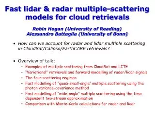
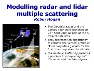
Modelling radar and lidar multiple scatteringRobin Hogan The CloudSat radar and the Calipso lidar were launched on 28th April 2006 as part of the A-train of satellites They represent an opportunity to retrieve the vertical profile of cloud properties globally for the first time: important for climate But multiple scattering presents a problem in interpreting both the radar and the lidar signals
7 June 2006 Aerosol from China? Molecular scattering Non-drizzling stratocumulus Cirrus Mixed-phase altocumulus Drizzling stratocumulus Rain • Calipso lidar (l<r) • CloudSat radar (l>r) 5500 km Japan Eastern Russia East China Sea Sea of Japan
1D variational method New ray of data First guess of x • In this problem, the observation vector y and state vector x are: Forward model Predict measurements y and Jacobian H from state vector x using forward modelH(x) Compare measurements to forward model Has the solution converged? 2 convergence test No Gauss-Newton iteration step Predict new state vector: xi+1= xi+A-1{HTR-1[y-H(xi)] +B-1(b-xi)} where the Hessian is A=HTR-1H+B-1 Yes Calculate error in retrieval The solution error covariance matrix is S=A-1 Proceed to next ray
Examples of multiple scattering • LITE lidar on the space shuttle in 1994 • Large detector footprint (300 m) means that photons may be scattered many times and still remain within the field-of-view • The long path-length means that those detected appear to have been scattered back from below cloud base (or below the surface) • Need a sophisticated lidar forward model to represent this Stratocumulus Surface echo (sea) Apparent echo from below the sea surface!
Multiple scattering Multiple scattering CloudSat radar Bangladesh Bay of Bengal MODIS infrared image Bangladesh Himalayas
Intense convection over the Amazon Multiple scattering
Multiple scattering so strong it corrupts next ray, appearing above the cloud!
Phase functions • Radar & cloud droplet • l >> D • Rayleigh scattering • g ~ 0 • Radar & rain drop • l ~ D • Mie scattering • g ~ 0.5 • Lidar & cloud droplet • l << D • Mie scattering • g ~ 0.85 Asymmetry factor Q q
Scattering regimes • Regime 2: Quasi-small-angle multiple scattering • Ql~ x • Only for wavelength much less than particle size • Lidar & ice clouds • Regime 3: Full multiple scattering • l~ x Mean free path l • Regime 0: No attenuation • Optical depth << 1 • mm-wave radar & ice cloud • Lidar & optically thin aerosol • Regime 1: Single scattering • mm-wave radar & liquid cloud • Lidar & optically thick aerosol Footprint x
New algorithm • Use the Hogan (Applied Optics, 2006) algorithm for the “quasi-direct” return (contribution from regimes 1 and 2) • Use the “time-dependent two-stream” approximation for wide-angle multiple scattering (regime 3) Space-time diagram
Quasi-small-angle multi-scattering Wide field-of-view: forward scattered photons may be returned Narrow field-of-view: forward scattered photons escape • To calculate the “quasi-direct” component: • Eloranta’s (1998) model • O (N m/m !) efficient for N points in profile and m-order scattering • Too expensive to take to more than 3rd or 4th order in retrieval (not enough) • Hogan (2006)method treats third and higher orders together • O (N 2) efficient • As accurate as Eloranta when taken to ~6th order • 3-4 orders of magnitude faster for N =50 (~ 0.1 ms) Ice cloud Molecules Liquid cloud Aerosol Hogan (Applied Optics, 2006). Code: www.met.rdg.ac.uk/clouds
Time-dependent two-stream approx. • Describe diffuse flux in terms of outgoing stream I+ and incoming stream I-, and numerically integrate the following coupled PDEs: • These can be discretized using simple schemes in time and space, provided that the optical depth of each layer is small Source Scattering from the quasi-direct beam into each of the streams Time derivative Remove this and we have the time-independent two-stream approximation used in weather models Gain by scattering Radiation scattered from the other stream Spatial derivative A bit like an advection term, representing how much radiation is upstream Loss by absorption or scattering Some of lost radiation will enter the other stream
Lateral photon spreading • Two-stream equations are inherently 1D, so can’t predict the lateral spreading of photons that is necessary to determine the fraction of them remaining within the instrument field-of-view • Solution: model the lateral variance of photon position, , using the following equations (where ): • Then assume the lateral photon distribution is Gaussian to predict what fraction of it lies within the field-of-view Additional source Increasing variance with time is described by a diffusivity D
Simulation of 3D photon transport • Scalar (actinic) flux is shown (I++I-) • Colour scale is logarithmic • Represents 5 orders of magnitude • Domain properties: • 500-m thick • 2-km wide • Optical depth of 20 • No absorption • In this simulation the lateral distribution is Gaussian at each height and each time
Comparison with Monte Carlo • Very good agreement found with Monte Carlo (much slower!) for simple cloud case and a wide range of fields-of-view Monte Carlo calculation courtesy of Tamas Varnai (NASA) for an I3RC case (Intercomparison of 3D Radiation Codes)
Effect on integrated backscatter • Need to be careful in applying the O’Connor et al. (2004) calibration technique for wide field-of-view lidars; may no longer asymptote • It is possible that integrated backscatter could provide information on optical depth
Future work • Modify the numerics so that discretizations can be used where the optical depth is large within one layer • Find a way to estimate the Jacobian so that the new forward model can be applied in a variational retrieval scheme • Implement in the CloudSat/Calipso retrieval scheme • More confidence in lidar retrievals in liquid water clouds • Can interpret CloudSat returns in deep convection • Apply to multiple field-of-view lidars • The difference in backscatter for two different fields of view enables the multiple scattering to be quantified and interpreted in terms of cloud properties • Predict the polarization of the returned signal • Difficult, but useful for lidar because multiple scattering depolarizes the return in liquid water clouds which would otherwise not depolarize