Download

1 / 17
170 likes | 353 Views
Final Review Biost / Epi 536 . December 14, 2009. Outline. Before the midterm: Interpretation of model parameters (Cohort vs case-control studies) Hypothesis testing Adjusting for confounding Exposure modeling. Outline. Since the midterm: Interaction DAGs Omitted covariates

E N D
Final ReviewBiost/Epi 536 December 14, 2009
Outline • Before the midterm: • Interpretation of model parameters • (Cohort vs case-control studies) • Hypothesis testing • Adjusting for confounding • Exposure modeling
Outline • Since the midterm: • Interaction • DAGs • Omitted covariates • Assessing model fit (influential observations: notes p370-389) • Advanced coding • Conditional logistic regression • Conditional vs Marginal adjustment • Conditional vs Marginal causal models • Marginal structural models (briefly) • Prediction (briefly)
Interaction • Many possible forms • Confirmatory: include as spec’d in prior hypothesis • Exploratory: include interactions that have a priori rationale and find best-fitting, succinct form • Rules • Interaction and main effect can have different forms • Interaction should be nested within main effect • (HW 10 key, notes p260-300)
DAGs C E D • DAGs help us visualize confounding • Confounding occurs when there are unblocked backdoor paths between E and D • Backdoor paths may be blocked by: • Colliders • Controlling for variables • Sufficient: a set of variables that • control for confounding • Minimally sufficient: smallest sufficient set • (HW 11 key, notes p301-342) F B G
Omitted covariates: take-home message • Adding an additional variable X to a logistic model will ALWAYS change the interpretation of the coefficient for the exposure of interest. • Why? OR compares two values with the same value of X (conditional OR) rather than randomly chosen individuals (marginal OR). • Marginal OR != Conditional OR • When X is strongly associated with E or D, controlling for X can reduce the precision to estimate the log OR and reduce the power of the test for the exposure parameter
Advanced Coding • Many examples: • Genetics (HW 14) • Nutritional epi (HW 13, pop quiz) • Notes p357-369 • Take-home message: • Interpretation depends on the coding of both the variable of interest and other variables in the model. • “Other variables held constant” doesn’t always make sense. • When in doubt, write out logits.
Conditional Logistic Regression • Method of estimation (conditional likelihood) • Estimates are interpreted as in normal logistic regression • Use to reduce bias when you have many nuisance parameters (example: matched sets) • Stratum-specific parameters aren’t estimated, but stratum variables are in the model • Can only estimate coefficients for covariates that vary w/in at least one stratum (HW 15-16, notes p423-449)
Conditional vs. Marginal Causal Models • Goal: Control confounding. Method depends on parameter of interest. • Subject-specific • “How much more likely is a person to get the disease if they are exposed?” • Regression can be useful here • Population average • Compare average risk of disease in the population if everyone is exposed, vs. if no one was exposed • Example: causal effect of population interventions • Regression not useful here (Notes p398-422)
Conditional vs. Marginal Causal Models • Homogeneous pop/subpop: pop/subpop parameters have subject-specific interpretation • In general: if estimating P(disease|exp+) – P(disease|exp-), can estimate avg causal effect for pop/subpop • In case-control studies: can’t estimate this difference! Can estimate pop/subpop ORs. With strong assumptions, we can say subpop ORs are avg subject-specific ORs.
Conditional vs. Marginal Causal Models • Logistic regression • Covariates define subpopulations • Estimate pop/subpop level causal effects when there is no confounding • Can’t control subpop confounding reliably • Control confounding for average subject-specific causal effects when subpops defined by strata are homogeneous (strong assumption) • Include variables related to disease (not necessarily confounders)
Conditional vs. Marginal Adjustment • Conditional: compare similar individuals • Common OR using logistic regression/M-H • We’ve done this a lot! • Marginal: compare individuals randomly selected from a population • Reweight exposure probabilities so cases and controls have same confounder distribution, then calculate OR. • Standardization • Marginal structural models • Conditional and marginal ORs will be different (Notes p390-397)
Conditional vs. Marginal Adjustment • Crude OR uses confounded P(Exposed) for cases and controls: • SUM[ P(C=ci) x P(Exposed|C=ci) ] • Exposure probabilities are weighted differently b/c of different confounder distributions for cases and controls • Conditional OR: Same exposure OR within confounder strata
Conditional vs. Marginal Adjustment • Marginal OR uses adjusted P(Exposed) for cases and controls: • SUM[ P(control, C=ci) x P(Exposed|C=ci) ] • Weighting distribution of C in cases to match distribution in controls • Marginal structural models also standardize pop-level ORs • Weights: Proportion of observations that would be in the sample for C=c and E=e if C and E weren’t related • (MSM: Notes p450-465)
Conditional vs. Marginal Adjustment • Marginal • Could standardize to any population • Estimate is not conditional on value of confounding variable • Interpretation of OR depends on population chosen • Look at the association of interest comparing populations with different exposure levels, but each with the same distribution of the confounding variable. • Conditional • Better for subpopulation-level ORs • Subpop ORs can sometimes be interpreted as subject-level • Look at the association of interest comparing individuals with different exposure levels but with the same level of the confounding variable.
Prediction • Goal: Develop a rule to predict outcomes • Method • Using training data, develop predictive models and obtain parameter estimates. • Using validation data, pick the best model. • Using test data, estimate prediction error associated with the best model. • (We can fudge this a little but this is the best method.)