Download
1 / 28
280 likes | 534 Views
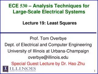
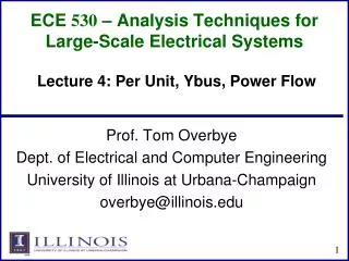
ECE 530 – Analysis Techniques for Large-Scale Electrical Systems. Lecture 17: Sensitivity Analysis. Prof. Tom Overbye Dept. of Electrical and Computer Engineering University of Illinois at Urbana-Champaign overbye@illinois.edu. Announcements. HW 6 will be assigned next time

E N D
ECE 530 – Analysis Techniques for Large-Scale Electrical Systems Lecture 17: Sensitivity Analysis Prof. Tom Overbye Dept. of Electrical and Computer Engineering University of Illinois at Urbana-Champaign overbye@illinois.edu
Announcements • HW 6 will be assigned next time • Midterm exam average was 83.6; high score was 96
Sensitivity Analysis • Previously with the standard assumption that the power flow Jacobian is nonsingular, we have • We can then compute the change in the line real power flow vector
Previous Notation • The series admittance of line is g+jb and we define • Recall we defined the LN incidence matrix where the component j of ai isnonzero whenever line i iscoincident with node j. Hence A is quite sparse, with two nonzeros per row
Linearized Sensitivity Analysis • By using the approximations from the fast decoupled power flow we can get sensitivity values that are independent of the current state. That is, by using the B' and B" matrices • For line flow we can approximate
Linearized Sensitivity Analysis • Also, for each line and so, (the negative sign goes away because of how we defined )
Linearized Active Power Flow Model • Under these assumptions the change in the real power line flows are given as • The constant matrix is called the injection shift factor matrix (ISF)
Injection Shift Factors (ISFs) • The element in row and column n of is called the injection shift factor (ISF)of line with respect to the injection at node n • Absorbed at the slack bus, so it is slack bus dependent • Terms generation shift factor (GSF) and load shift factor (LSF) are also used • Same concept, just a variation in the sign whether it is a generator or a load • Sometimes the associated element is not a single line, but rather a combination of lines (an interface) • Terms used in North America are defined in the NERC glossary (http://www.nerc.com/files/glossary_of_terms.pdf)
ISF : Interpretation is the fraction of the additional 1MW injection at node n that goes though line slack node
ISF : Properties • By definition, depends on the location of the slack bus • By definition, for since the injection and withdrawal buses are identical in this case and, consequently, no flow arises on any line • The magnitude of is at most 1 since Note, this is strictly true only for the linear (lossless)case. In the nonlinear case, it is possible that atransaction decreases losses so a 1 MW injectionchanges a line flow by more than 1 MW.
Five Bus Example The row of Acorrespond to thelines and transformers, the columns correspondto the non-slack buses (buses 2 to 5);for each line thereis a 1 at one end, a -1 at the other end(hence an assumedsign convention!); herewe put a 1 for the lowernumbered bus
Five Bus Example Comments • At first glance the numerically determined value of (128-118)/20=0.5 does not match closely with the analytic value of 0.5455; however, in doing the subtraction we are losing numeric accuracy • Adding more digits helps (128.40 – 117.55)/20 = 0.5425 • The previous matrix derivation isn’t intended for actual computation; is a full matrix so we would seldom compute all of its values • Sparse vector methods can be used if we are only interested in the ISFs for certain lines and certain buses
Distribution Factors • Various additional distribution factors may be defined • power transfer distribution factor (PTDF) • line outage distribution factor (LODF) • line closure distribution factor (LCDF) • outage transfer distribution factor (OTDF) • These factors may be derived from the ISFs making judicious use of the superposition principle
Definition: Basic Transaction • A basic transaction involves the transfer of a specified amount of power t from an injection node m to a withdrawal node n
Definition: Basic Transaction • We use the notation to denote a basic transaction injection node withdrawal node quantity
Definition: PTDF • NERC defines a PTDF as • “In the pre-contingency configuration of a system under study, a measure of the responsiveness or change in electrical loadings on transmission system Facilities due to a change in electric power transfer from one area to another, expressed in percent (up to 100%) of the change in power transfer” • Transaction dependent • We’ll use the notation to indicate the PTDF on line with respect to basic transaction w • In the lossless formulation presented here (and commonly used) it is slack bus independent
PTDFs Note, the PTDF is independentof the amount t;often expressed asa percent
Calculating PTDFs in PowerWorld • PowerWorld provides a number of options for calculating and visualizng PTDFs • Select Tools, Sensitivities, Power Transfer Distribution Factors (PTDFs) Results areshown for thefive bus casefor the Bus 2 to Bus 3 transaction
PowerWorld PTDF Visualization • To visualize the PTDFs, right click on the one-line background and, Animated Flows • Select Oneline Display Options and then set the Base Flow Scaling on PTDF Percentage Flows • Select Pie Chart/Gauges and change Pie Chart Style to PTDF, set the Show Percent to a small value, like 1%
Five Bus PTDF Visualization PowerWorld Case: B5_DistFact_PTDF
Nine Bus PTDF Example Display showsthe PTDFsfor a basictransactionfrom Bus Ato Bus I. Notethat 100% ofthe transactionleaves Bus Aand 100%arrives at Bus I PowerWorld Case: B9_PTDF
Eastern Interconnect Exmaple: Wisconsin Utility to TVA PTDFs In thisexamplemultiplegeneratorscontributefor both the sellerand thebuyer Contours show lines that would carry at least 2% of a power transfer from Wisconsin to TVA
Line Outage Distribution Factors (LODFs) • Power system operation is practically always limited by contingencies, with line outages comprising a large number of the contingencies • Desire is to determine the impact of a line outage (either a transmission line or a transformer) on other system real power flows without having to explicitly solve the power flow for the contingency • These values are provided by the LODFs • The LODF is the portion of the pre-outage real power line flow on line k that is redistributed to line as a result of the outage of line k