Large Scale DNA Sequence Analysis and Biomedical Computing using MapReduce , MPI and Threading
Large Scale DNA Sequence Analysis and Biomedical Computing using MapReduce , MPI and Threading. Judy Qiu xqiu@indiana.edu www.infomall.org/salsa Community Grids Laboratory, Digital Science Center Indiana University. Workshop on Enabling Data-Intensive Computing: from Systems to Applications


Large Scale DNA Sequence Analysis and Biomedical Computing using MapReduce , MPI and Threading
E N D
Presentation Transcript
Large Scale DNA Sequence Analysis and Biomedical Computing using MapReduce, MPI and Threading Judy Qiu xqiu@indiana.eduwww.infomall.org/salsa • Community Grids Laboratory, • Digital Science CenterIndiana University Workshop on Enabling Data-Intensive Computing: from Systems to Applications July 30-31, 2009, Pittsburgh
Collaboration in SALSAProject Microsoft Research Technology Collaboration Dryad Roger Barga Christophe Poulain CCR (Threading) George Chrysanthakopoulos DSS HenrikFrystykNielsen • Indiana University • SALSATeam Geoffrey Fox Xiaohong Qiu Scott Beason • JaliyaEkanayake • ThilinaGunarathne • ThilinaGunarathne JongYoulChoi Yang Ruan • Seung-Hee Bae Others ApplicationCollaboration Bioinformatics, CGB Haiku Tang, Mina Rho, Peter Cherbas, Qunfeng Dong IU Medical School Gilbert Liu Demographics (GIS) Neil Devadasan Cheminformatics Rajarshi Guha (NIH), David Wild Physics CMS group at Caltech (Julian Bunn) • Community Grids Lab • and UITS RT – PTI
Data Intensive (Science) Applications • 1) Data starts on some disk/sensor/instrument • It needs to bepartitioned; often partitioning natural from source of data • 2) One runs a filterof some sort extracting data of interest and (re)formatting it • Pleasingly parallel with often “millions” of jobs • Communication latencies can be many millisecondsand can involve disks • 3) Using same (or map to a new) decomposition, one runs a parallel application that could require iterative steps between communicating processes or could be pleasing parallel • Communication latencies may be at most some microsecondsand involves shared memory orhigh speed networks • Workflow links 1) 2) 3) with multiple instances of 2) 3) • Pipeline or more complex graphs • Filters are “Maps” or “Reductions” in MapReduce language
“File/Data Repository” Parallelism Instruments Map = (data parallel) computation reading and writing data Reduce = Collective/Consolidation phase e.g. forming multiple global sums as in histogram Communication via Messages/Files Portals/Users Map1 Map2 Map3 Reduce Disks Computers/Disks
Data Analysis Examples • LHC Particle Physics analysis: File parallel over events • Filter1:Process raw event data into “events with physics parameters” • Filter2:Process physics into histograms using ROOT or equivalent • Reduce2: Add together separate histogram counts • Filter 3: Visualize • Bioinformatics - Gene Families: Data parallel over sequences • Filter1: Calculate similarities (distances) between sequences • Filter2: Align Sequences (if needed) • Filter3: Cluster to find families and/or other statistical tools • Filter 4:Apply Dimension Reduction to 3D • Filter5:Visualize
Particle Physics (LHC) Data Analysis MapReduce for LHC data analysis LHC data analysis, execution time vs. the volume of data (fixed compute resources) • Root running in distributed fashion allowing analysis to access distributed data
Reduce Phase of Particle Physics “Find the Higgs” using Dryad • Combine Histograms produced by separate Root “Maps” (of event data to partial histograms) into a single Histogram delivered to Client
Notes on Performance • Speed up = T(1)/T(P) = (efficiency ) P with P processors • Overhead f= (PT(P)/T(1)-1) = (1/ -1)is linear in overheads and usually best way to record results if overhead small • For MPI communicationf ratio of data communicated to calculation complexity = n-0.5 for matrix multiplication where n (grain size) matrix elements per node • MPI Communication Overheads decrease in sizeas problem sizes n increase (edge over area rule) • Dataflow communicates all data – Overhead does not decrease • Scaled Speed up: keep grain size n fixed as P increases • Conventional Speed up: keep Problem size fixed n 1/P • VMs and Windows Threads have runtime fluctuation /synchronization overheads
Gene Sequencing Application • This is first filter in Alu Gene Sequence study – find Smith Waterman dissimilarities between genes • Essentially embarrassingly parallel • Note MPI faster than threading • All 35,229 sequences require 624,404,791 pairwise distances = 2.5 hours with some optimization • This includes calculation and needed I/O to redistribute data) Parallel Overhead =(Number of Processes/Speedup) - 1 Two data set sizes
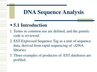
Some Other File Parallel Examplesfrom Indiana University Biology Dept. • EST (Expressed Sequence Tag) Assembly: 2 million mRNA sequences generates 540000 files taking 15 hours on 400 TeraGrid nodes (CAP3 run dominates) • MultiParanoid/InParanoid gene sequence clustering: 476 core years just for Prokaryotes • Population Genomics: (Lynch) Looking at all pairs separated by up to 1000 nucleotides • Sequence-based transcriptome profiling: (Cherbas, Innes) MAQ, SOAP • Systems Microbiology (Brun) BLAST, InterProScan • Metagenomics (Fortenberry, Nelson) Pairwise alignment of 7243 16s sequence data took 12 hours on TeraGrid • All can use Dryad
CAP3 Results • Results obtained using using two clusters running at IU and Microsoft. Each cluster has 32 nodes and so each node has 8 cores. There is a total of 256 cores. • Cap3 is a sequence assembly program that operates on a collection of gene sequence files which produce several output files. • In parallel implementations, the input files are processed concurrently and the outputs are saved in a predefined location. • As a comparison, we have implemented this application using Hadoop, CGL-MapReduce (enhanced Hadoop) and Dryad.
CAP3 Results Number of CAP3 Files
Files Files Files Files Files Files Data Intensive Architecture InstrumentsUser Data Visualization User Portal Knowledge Discovery Users InitialProcessing Higher LevelProcessing Such as R PCA, Clustering Correlations … Maybe MPI Prepare for Viz MDS
Why Gather/ Scatter Operation Important • There is a famous factor of 2 in many O(N2) parallel algorithms • We initially calculate in parallel Distance(i,j) between points (sequences) i and j. • Done in parallel over all processor nodes for say i < j • However later parallel algorithms may want specific Distance(i,j) in specific machines • Our MDS and PWClustering algorithms require each of N processes has 1/N of sequences and for this subset {i} Distance({i},j) for ALL j. i.e. wants both Distance(i,j) and Distance(j,i) stored (in different processors/disk) • The different distributions of Distance(i,j) across processes is in MPI called a scatter or gather operation. This time is included in previous SW timings and is about half total time • We did NOT get good performance here from either MPI (it should be a seconds on Petabit/sec Infiniband switch) or Dryad • We will make needed primitives precise and greatly improve performance here
High Performance Robust Algorithms • We suggest that the data deluge will demand more robust algorithms in many areas and these algorithms will be highly I/O and compute intensive • Clustering N= 200,000 sequences using deterministic annealing will require around 750 cores and this need scales like N2 • NSF Track 1 – Blue Waters in 2011 – could be saturated by 5,000,000 point clustering
High end Multi Dimension scaling MDS • Given dissimilarities D(i,j), find the best set of vectors xi in d (any number) dimensions minimizing i,j weight(i,j) (D(i,j) – |xi – xj|n)2 (*) • Weight chosen to refelect importance of point or perhaps a desire (Sammon’s method) to fit smaller distance more than larger ones • n is typically 1 (Euclidean distance) but 2 also useful • Normal approach is Expectation Maximation and we are exploring adding deterministic annealing to improve robustness • Currently mainly note (*) is “just” 2 and one can use very reliable nonlinear optimizers • We have good results with Levenberg–Marquardt approach to 2 solution (adding suitable multiple of unit matrix to nonlinear second derivative matrix). However EM also works well • We have some novel features • Fully parallel over unknowns xi • Allow “incremental use”; fixing MDS from a subset of data and adding new points • Allow general d, n and weight(i,j) • Can optimally align different versions of MDS (e.g. different choices of weight(i,j) to allow precise comparisons • Feeds directly to powerful Point Visualizer
Deterministic Annealing Clustering • Clustering methods like Kmeans very sensitive to false minima but some 20 years ago an EM (Expectation Maximization) method using annealing (deterministic NOT Monte Carlo) developed by Ken Rose (UCSB), Fox and others • Annealing is in distance resolution – Temperature T looks at distance scales of order T0.5. • Method automatically splits clusters where instability detected • Highly efficient parallel algorithm • Points are assigned probabilities for belonging to a particular cluster • Original work based in a vector space e.g. cluster has a vector as its center • Major advance 10 years ago in Germany showed how one could use vector free approach – just the distances D(i,j) at cost of O(N2) complexity. • We have extended this and implemented in threading and/or MPI • We will release this as a service later this year followed by vector version • Gene Sequence applications naturally fit vector free approach.
Key Features of our Approach • Initially we will make key capabilities available as services that we eventually be implemented on virtual clusters (clouds) to address very large problems • Basic Pairwise dissimilarity calculations • R (done already by us and others) • MDS in various forms • Vector and Pairwise Deterministic annealing clustering • Point viewer (Plotviz) either as download (to Windows!) or as a Web service • Note all our code written in C# (high performance managed code) and runs on Microsoft HPCS 2008 (with Dryad extensions)
Various Alu Sequence Resultsshowing Clustering andMDS 3000 Points : Clustal MSAKimura2 Distance 4500 Points : Pairwise Aligned 4500 Points : Clustal MSA Map distances to 4D Sphere before MDS
Pairwise Clustering of 35229 Sequences Initial Clustering of 35229 Sequences showing first four clusters identified with different colors The Pairwise clustering using MDS on same sample to display results. It used all 768 cores from Tempest Windows cluster Further work will improve clustering. Investigate sensitivity to alignment (Smith Waterman) and give performance details
PWDA Parallel Pairwise data clustering by Deterministic Annealing run on 24 core computer ParallelOverhead Intra-nodeMPI Inter-nodeMPI Threading Parallel Pattern (Thread X Process X Node)
Parallel Pairwise Clustering PWDA Speedup Tests on eight 16-core Systems (6 Clusters, 10,000 Patient Records) Threading with Short Lived CCR Threads Parallel Overhead Parallel Patterns (# Thread /process) x (# MPI process /node) x (# node)
MDS and Primary PCA Vector • MDS of 635 Census Blocks with 97 Environmental Properties • Shows expected Correlation with Principal Component – color varies from greenish to reddish as projection of leading eigenvector changes value • Ten color bins used
Canonical Correlation • Choose vectors a and b such that the random variables U = aT.Xand V = bT.Ymaximize the correlation = cor(aT.X,bT.Y). • X Environmental Data • Y Patient Data • Use R to calculate = 0.76
MDS and Canonical Correlation • Projection of First Canonical Coefficient between Environment and Patient Data onto Environmental MDS • Keep smallest 30% (green-blue) and top 30% (red-orchid) in numerical value • Remove small values < 5% mean in absolute value
References • K. Rose, "Deterministic Annealing for Clustering, Compression, Classification, Regression, and Related Optimization Problems," Proceedings of the IEEE, vol. 80, pp. 2210-2239, November 1998 • T Hofmann, JM BuhmannPairwise data clustering by deterministic annealing, IEEE Transactions on Pattern Analysis and Machine Intelligence 19, pp1-13 1997 • HansjörgKlockand Joachim M. BuhmannData visualization by multidimensional scaling: a deterministic annealing approachPattern Recognition Volume 33, Issue 4, April 2000, Pages 651-669 • Granat, R. A., Regularized Deterministic Annealing EM for Hidden Markov Models, Ph.D. Thesis, University of California, Los Angeles, 2004. We use for Earthquake prediction • Geoffrey Fox, Seung-HeeBae, JaliyaEkanayake, XiaohongQiu, andHuapeng Yuan, Parallel Data Mining from Multicore to Cloudy Grids, Proceedings of HPC 2008 High Performance Computing and Grids Workshop, Cetraro Italy, July 3 2008 • Project website: www.infomall.org/salsa