Download
1 / 27
270 likes | 405 Views
Status of component 4, “urbanLS”… testing the four optional configurations (forward/backward, 0 th /1 st order). John Wilson, 22 August/06. Context Random Displacement Model is it well-mixed? does it agree with standard dispersion data?

E N D
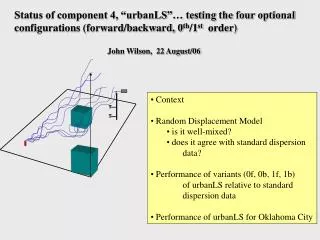
Status of component 4, “urbanLS”… testing the four optional configurations (forward/backward, 0th/1st order) John Wilson, 22 August/06 • Context • Random Displacement Model • is it well-mixed? • does it agree with standard dispersion data? • Performance of variants (0f, 0b, 1f, 1b) of urbanLS relative to standard dispersion data • Performance of urbanLS for Oklahoma City
Context: High resolution weather analysis/prediction: “Urban GEM-LAM” Provides upwind and upper boundary conditions Building-resolving k- turbulence model: “urbanSTREAM” (steady state, no thermodynamic equation, control volumes congruent with walls) Provides computational mesh over flow domain and these gridded fields: Lagrangian stochastic model “urbanLS” to compute ensemble of paths from source(s); now offers four options 0f, 0b, 1f, 1b
Why is the RDM of interest? • A zeroth-order Lagrangian stochastic model, also called the “Random Displacement Model” (RDM), does not explicitly model particle velocity, and (by some criteria) is equivalent to an eddy-diffusion treatment… however it is a Lagrangian method, thus grid free • It is far less demanding, computationally, than the 1st-order LS model… and in the far field of a source, the RDM/eddy diffusion treatment is acceptable… as I will demonstrate here
The complexity of a 1st - order order LS algorithm… ( G a standardized Gaussian random variate) The T’s involve the mean velocity field, TKE dissipation rate , and the stress tensor Rij . They are computed and stored on the grid prior to computing the ensemble of paths. At each timestep, use T’s from gridpoint closest to particle (ie. no interpolation to particle position)
Relative simplicity of the 0th - order LS algorithm where and no requirement that • Attractive to use 0th-order LS for its speed. Criteria: • is the algorithm well-mixed? • does it replicate standard experiments? Will address these questions in context of simplest real world (atmospheric) regime of flow, viz., neutral surface layer
“Well-mixed”? t > 0 t = 0 uniform initial density “p” Still uniform?
zsrc = 0.46 m 100 m Reference dispersion data traceable back to Project Prairie Grass Ideal neutral surface layer (no horiz. gradients) Detect crosswind-integrated concentration 9 min
universal function of x/z0 z/z0
Form of the RDM (0th-order LS) for neutral surface layer Forward model m=1 Do we reverse this (m = -1) in a backward model?
Analytical and numerical tests for well-mixed property (nb! grid-free LS algorithm) Chapman-Kolmogorov equation: “transition density” Final state Upper and lower reflection boundaries Initial state (= 1 for present test)
Analytical and numerical tests for well-mixed property no reflection: path length reflection path has total length where 14.5 min
RDM with surface reflection is not a well-mixed model Flow regime: ideal neutral surface layer L = Upper reflection at L=4000 z0 Lower reflection at zr=0
… but it (RDM) gives excellent simulation of reference dispersion “True” normalized, crosswind-integrated concentration at x/z0=2000 is 1.48 x 10⁻³
And treatment of the drift term?.... “Truth”… do not reverse drift term
Now test actual code (urbanLS3.for) against reference dispersion by scaling PPG onto the urbanSTREAM grid for Oklahoma City: at its highest resolution, z=3 m (x, y irrelevant since horizontal gradients vanish) • urbanLS is not a grid-free Lagrangian model; unless the grid resolves the strong near-ground gradients of the ASL precise forward/backward 0/1-order consistency should not be expected; if one simulates (eg.) PPG57 with z0= 0.006 m on this grid at full scale , then the velocity statistics in the lowest layer (k=2) represent the flow in the range • therefore specify z0=zc(2)/2=0.75 m and a source-detector separation of 2000z0 scales to 1500 m. Discretization error is greatly reduced, because the wind statistics in the plume layer are represented by more than 50 layers • perfect reflection at zrefl=z0
x (I) Timestep 1st-order simulations: 0th-order simulations:
0th-order forward simulation excellent; backward very sensitive to t • forward-backward consistency of 1st order simulations • only modest sensitivity to timestep, but do need t/TL smaller than 0.1 to attain agreement within one std error with reference dispersion data • bigger impact of t on backward than forward simulation
Focus on 0th-order simulations: • forward simulation good, and not very sensitive to whether one sets drift term to zero in lowest layer • backward simulation very sensitive to whether drift term is reversed, to whether it is zeroed in lowest layer, and to t
Recapitulate implications of tests of 0f, 0b, 1f, 1b against reference dispersion case: • 1st-order forward and backward consistent, in good agreement with the reference dispersion data, only weakly sensitive to t • 0th-order forward simulation in good agreement with the reference dispersion data, even with large t, and only weakly sensitive to inclusion or neglect of drift term in lowest layer • 0th-order backward simulation demands drift term should not be reversed, but should be zeroed in lowest layer… else spurious vertical gradient arises • remains to comprehend the 0th-order backward simulations, which for the time being I distrust 26.5 min
Simulation of Gas Plume from a source in Oklahoma City Intensive Observation Period 9, July 27, 2003: 0615-0630 continuous source 1.9 m above ground wind
350 m wind (Not to scale) #74 200 forward paths, displayed only below 50 m height
Mean ground-level concentration [parts per trillion] from forward LS simulation • fully 3D, C0=4.8 • dt = 0.05 min (TL, x/u ) • zrefl=0.1 m • reset veloc. fluc if > 6 • 9 x 80,000 paths • detector half-widths 20 x 20 x 1.75 m • execution time 44 hrs • (3.68 min per 1000 paths)
Performance of (1f) Lagrangian model relative to experiment #74
Comparison of performance of (1f) Lagrangian and Eulerian solutions relative to experiment… Mean concentration [ppt]
Conclusion • evidence suggests 0f option in urbanLS is fast and reliable • puzzles remain relative to 0b option • remains to repeat the 0f, 0b, 1f, 1b consistency tests in disturbed flow • evidence suggests 0f, 1f, 1b options are all very satisfactory for realistic urban simulations • however no evidence yet that implementing Lagrangian approach driven by urbanSTREAM wind statistics offers any greater (or lesser) accuracy than Eulerian approach available in urbanSTREAM 31.5 min