HAJAR MOUNTAIN EXPERIMENT Convection and Precipitation over the Hajar mountains. (Juma Al-Maskari)

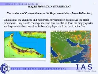
1. HAJAR MOUNTAIN EXPERIMENT Convection and Precipitation over the Hajar mountains. (Juma Al-Maskari) What causes the enhanced and catastrophic precipitation events over the Hajar mountains? Large scale convergence, heat low circulation form the empty quarter and large scale advection of moist boundary layer air from the Arabian Sea

2. In the wet-case, the sea-breeze converges with moisture flow advected from the Arabian Sea. This flow was also confirmed by sodar observations. Surface observations of dew-point temperature and wind speed and direction for Adam station and for Seeb station are also in agreement with the streamlines and the sodar winds. Examining various case studies indicated that the position of the heat low and its depth determine the direction and type of winds that converge over the mountains. A dry desert air (even when flowing over the Arabian Gulf) will lead to moist convection being suppressed, whereas moist air advected from the Arabian Sea will enhance moist convection. Moisture advection from the Arabian Sea in a column of at least 1 km depth is required for proper convection. The stronger the flow from the Arabian Sea and the deeper the column of the moist air, the heavier the precipitation. Results from the anelastic model show that the model is able to simulate cloud development and precipitation reasonably well, but the model seems to precipitate 2-3 hours earlier than observed. The model also shows that clouds develop over the mountain peaks and dissipate as they move west, which agrees well with radar and satellite imagery

3. Open boundary conditions Grid-box of 192 x 150 x 50 for dx=dy=2km and dz=400m, dt=4 sec. (also with dx=1km & dx=4km) Simulations were for 17 hours starting 4 am local, dumping every 10 minutes. An idealised surface heat flux forcing was introduced after 2 hours of model run. Variety sensitivity tests: dx=1km & dx=4km; variable grid resolution; variable moisture fields; reduction to10% fit orography; sea breeze sensitivity

4. Conclusions Sea-breeze, orographic forcing, moisture advection (and the depth of the moist column) from the Arabian Sea, and convergence are key factors in convective cloud development over the Hajar Mountains. The position of the thermal low and its depth determined whether the flow towards the mountains was dry desert or moist air from the Arabian Sea. Moisture advection from the Arabian Sea was the main ingredient for convection. The model demonstrated its ability to simulate the convergence of winds and cloud (development and movement) well. Model total precipitation was also in agreement with observations.

5. Application of a non-hydrostatic meteorological model to flow and dispersion of tracers in a street canyon. • Alan Gadian, Alison Coals, Nick Dixon, Sarah-Jane Lock, • Piotr Smolarkiewicz* and Alison Tomlin • Leeds University & MMM NCAR* • Can we understand more about processes at the street canyon scale from Meteorological Numerical Models? • Can Gal-Chen – Immersed Boundary Methods be used with conventional equations sets to look at small scale turbulent processes? • What does the flow look like? • Ultimately, Can “we understand” properties of transport of bulk parameters e.g. helicity or concentration

6. This approach has been applied to pollution dispersion in street canyons (1m resolution) and hills has been created (example wind and pollution concentration in Gillygate York). The images produced will correspond to vertical velocities and concentrations in the domain above defined by the dotted lines, with lamp-posts g3 and g4 marked

7. Figure 1. Schematic of the Gillygate canyon cross-section at G3-G4, showing relative locations of the five ultrasonic anemometers (Tomlin, 2008, QJRMS). Also indicated is a possible pathline for circulation when .

8. normalised by Mref Figure 6 (Tomlin, 2008) . Sector averaged in-street local turbulence intensity a) Anemometers on G3: , G3b; , G3m; ,G3t. b) Anemometers on G4: , G4m; , G4t; c) Anemometers at mid-height: , G3m; , G4m. Vertical whiskers indicate the 100 and 900 precentiles

9. Normalised t.k.e. against background wind direction for experimental data at a) G3 and b) G4. Experimental data show standard deviations of data as error bars (Dixon et al, 2005)

10. Non-hydrostatic LES models are widely used for meteorological forecasting. Although they can relatively slow compared with RANS simulations, they are able to describe accurately turbulent unsteady flow, eddy structures and transport of chemical species. These can include cloud and thermo-dynamical processes, will full feedback between the dynamics and thermodynamics with different stratification. Until recently these models have not been applicable in cases of steep orography and canyon flow, due to numerical difficulties with terrain following grid representations. Mathematical techniques now enable some of the computational and numerical issues to be overcome. Use of Gal-Chen terrain following co-ordinates with modified iterative solvers and alternative use of Immersed Boundary approach to simulate building structures will be demonstrated.

11. This presentation will analyse the flow in a street canyon in York, UK where observations were made with instruments located on lamp-posts (Dixon et al, 2006, Atmospheric Environment). Inter-comparison with model simulations from a modified form of a non-hydrostatic EULAG model (Grabowski & Smolarkiewicz, 2002, MWR,939-56) and Smolarkiewicz (2007, JCP) shows turbulence patterns. The results demonstrate the applicability of this approach to model high resolution flow and dispersion of, in this test case, inert tracers. The model has the advantage of being able to include the full range of dynamical and thermo-dynamical processes. The helical nature of the turbulent flow down the canyon is displayed. Further, a description of the venting of a simple line source of pollutant from the canyon base is shown. The effects and impact of street junctions on the vertical flux of pollutant is clearly demonstrated in the animations.

12. Terrain following co-ordinate models Can terrain following co-ordinates of flow over steep hills, street canyons work? Can the problems associated with anisotrophic cells be overcome? One such model is the Smolarkiewicz model, anelastic developed from the Clark-Hall code. Critical importance of pre-conditioner to obtain a solution for slopes over ~ 450. (Now implemented in models such as the Met Office UM) Gal-Chen (1975) terrain following co-ordinate system ( or sigma system in pressure co-ordinates ) For any function  , a Jacobian is needed to evaluate: LHS new co-odinate, RHS cartesian

13. Periodic domain, with uniform z0 = 0.1m Grid: 231 x 261 x 60 (tested at 80), for dx = dy = dz = 1m Model time: ~1200s , for dt = 0.025s Model spin up ~ 600s - results computed for a 1080s run, (1520-1680s) Rayleigh damping sponge above 50m Neutral, (constant dry potential temperature), u0= 5ms-1 from right to left. The periodic boundaries develop a logarithmic type surface layer. SGS and three simulations for calculation of mean and variances

14. Immersed Boundary (left) Gal Chen (right) lower boundary condition. Smolarkiewicz anelastic model, yz plot of vertical velocity w at 240s.

15. Two metre vertical velocity and concentration for the SE wind direction

16. Two metre vertical winds and concentrations for the NE wind direction

17. Two metre vertical winds and concentrations for the E wind direction

18. x-z and y-z cuts with Easterly wind direction

19. Conclusion: • The results have demonstrated a stable solution can be produced, which can • emulate the flow down a street canyon. The system, can be used to examine the • different thermal stability structures and variable wind fields • To be done: • Evaluate the modelled values of normalised turbulence and compare with observed data. Evaluate the statistical differences with the Gal-Chen and the Lower Immersed Boundary condition on the statistical flow • Calculate the helicity of the flow down the street canyon. Evaluate the product of the helicity and the concentration if pollutant. • Tabulate the efficiency of ventilation of the pollutant in the canyon, as a function of wind direction. • Plot normalised modelled concentrations with the data available.

21. Objectives: • To obtain as many observations as possible in order to validate the model’s ability to predict orographic convection. • To understand the important factors that enhances convection under certain conditions and suppresses it in others. • Figure 1 to the right shows positions of: • two sodars that were deployed just for this study (the sodars were alternated between 3 locations). • radiosondes that were launched from Seeb International Airport at 00,06, and • 12 UTC on selective days. • A Doppler radar located at Al-Ain in the United Arab Emirates which covers the western part of the model domain. (To complement radar data, imagery from geostationary satellite was used).