Multidimensional scaling MDS
Multidimensional scaling MDS. G. Quinn, M. Burgman & J. Carey 2003. Aim. Graphical representation of dissimilarities between objects in as few dimensions (axes) as possible. Graphical representation is termed an “ordination” in ecology

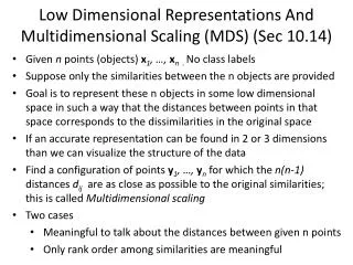
Multidimensional scaling MDS
E N D
Presentation Transcript
Multidimensional scalingMDS G. Quinn, M. Burgman & J. Carey 2003
Aim • Graphical representation of dissimilarities between objects in as few dimensions (axes) as possible
Graphical representation is termed an “ordination” in ecology • Axes of graph represent new variables which are summaries of original variables
Approximate distances by air (km) between Australian Capital cities CAN SYD MELB BRIS ADEL PER HOB DAR CAN 0 . . . . . . . SYD 246 0 . . . . . . MELB 506 727 0 . . . . . BRIS 1021 775 1393 0 . . . . ADEL 976 1185 651 1961 0 . . . PER 3126 3339 2804 4114 2152 0 . . HOB 1120 1075 613 1852 1264 3417 0 . DAR 3409 3163 3355 2886 2727 2951 4186 0
2 1 Dimension 2 0 -1 -2 -2 -1 0 1 2 Dimension 1 Stress = 0.014
2 Darwin 1 Brisbane Sydney Dimension 2 x -1 0 Canberra Melbourne Adelaide Hobart -1 Perth -2 -2 -1 0 1 2 Dimension 1
Darwin Brisbane Sydney Canberra Melbourne Adelaide Hobart Perth http://www.boardtheworld.com/resorts/country.php?cc=AU
Haynes & Quinn (unpublished) • Four sites along Morwell River • site 1 upstream from planned sewage outfall • sites 2, 3 and 4 downstream • site 3 below fish farm • Abundance of all species of invertebrates recorded from 3 stations at each site
12 objects (sampling units): • 4 sites by 3 stations at each site • 94 variables (species) Do invertebrate communities (or assemblages) differ between stations and sites? • Is Site 1 different from rest?
Multidimensional scaling 1. Set up a raw data matrix Species 1 2 3 4 5 etc. Site/sample S11 54 0 0 5 0 S12 37 1 0 4 0 S13 68 2 0 2 0 S21 60 0 0 0 1 S22 47 0 0 2 0 S23 60 0 0 0 0 etc.
2. Calculate a dissimilarity (Bray-Curtis) matrix S11 S12 S13 S21 S22 S23 etc. S11 .000 S12 .203 .000 S13 .666 .652 .000 S21 .216 .331 .759 .000 S22 .328 .410 .796 .191 .000 S23 .336 .432 .796 .183 .054 .000 etc.
3. Decide on number of dimensions (axes) for the ordination: • suspected number of underlying ecological gradients • match distances between objects on plot and dissimilarities between objects as closely as possible • more dimensions means better match • usually between 2 and 4 dimensions
4. Arrange objects (eg. sampling units) initially on ordination plot in chosen number of dimensions • starting configuration • usually generated randomly
Starting configuration 2 1 Axis II 0 -1 -2 -2 -1 0 1 2 Axis I Site 1 Site 2 Site 3 Site 4
5. Compare distances between objects on ordination plot and Bray-Curtis dissimilarities between objects • strength of relationship measured by Kruskal’s stressvalue • measures “badness of fit” so lower values indicate better match • plot is called Shepard plot
Distance Axis II 3 2 1 2 0 1 -1 -2 0 0 0.5 1 -2 -1 0 1 2 Axis I Dissimilarity Site 1 Site 2 Shepard plot Stress = 0.394 Site 3 Site 4 Starting configuration
6. Move objects on ordination plot iteratively by method of steepest descent • each step improves match between dissimilarities and distances between objects on ordination plot • lowers stress value
Axis II Distance 2 3 1 2 0 1 -1 -2 0 -2 -1 0 1 2 0 0.5 1 Axis I Dissimilarity After 20 iterations Stress = 0.119
7. Final configuration • further moving of objects on ordination plot cannot improve match between dissimilarities and distances • stress as low as possible
Axis I Distance 2 3 1 2 0 1 -1 -2 0 -2 -1 0 1 2 0 0.5 1 Axis II Dissimilarity Final configuration - 50 iterations Stress = 0.069
Iteration history Iteration Stress 1 0.394 2 0.368 3 0.357 4 0.351 ... ... 20 0.119 ... ... 49 0.069 50 0.069 Stress of final configuration is 0.069
How low should stress be? Clarke (1993) suggests: • > 0.20 is basically random • < 0.15 is good • < 0.10 is ideal • configuration is close to actual dissimilarities
How many dimensions? • Increasing no. of dimensions above 4 usually offers little reduction in stress • 2 or 3 dimensions usually adequate to get good fit (ie. low stress) • 2 dimensions straightforward to plot
Distance Dissimilarity Types of MDS • Based on how stress is measured • Relationship between distance and dissimilarity
Metric MDS • stress measured from relationship between actual dissimilarities and distances • but relationship often non-linear • inefficient?
Non-metric MDS • stress measured from relationship between ranks of dissimilarities and ranks of distances • similar to Spearman rank correlation • better for ecological data
Anderson et al. (1994) • Effects of substratum type on recruitment of intertidal estuarine fouling assemblage • Six replicate panels of 4 substrata placed in estuary for 1 month at 2 times of the year • 14 species in total recorded
MDS to examine relationship between panel • do substrata appear different in spp composition? • Bray-Curtis dissimilarity • Non-metric MDS
January October Stress = 0.126 Stress = 0.116 concrete plywood aluminium fibreglass
Comparing groups in MDS Haynes & Quinn data • 4 groups (sites) - must be a priori groups • 3 replicate stations per site (n = 3) • Are sites significantly different in species composition? • Is there an ANOVA-like equivalent for MDS?
Analysis of similarities - ANOSIM • Uses (dis)similarity matrix • Because dissimilarities are not normally distributed, uses ranks of pairwise dissimilarities • Because dissimilarities are not independent of each other, uses randomisation test rather than usual significance testing procedure • Generates own test statistic (called R) by randomisation of rank dissimilarities • Available through PRIMER package • Not SYSTAT nor SPSS
Average of rank dissimilarities between objects within groups = average of rank dissimilarities between objects between groups rB = rW No difference in species composition between groups Null hypothesis
Within group dissimilarities Between group dissimilarities
R average of rank dissimilarities between objects between groups - average of rank dissimilarities between objects within groups • R = (rB - rW) / (M / 2) where M = n(n-1)/2 • R between -1 and +1. • Use randomization test to generate probability distribution of R when H0 is true. Test statistic
Haynes & Quinn ANOSIM • R = 0.583, P = 0.002 so reject Ho. • Significant differences between sites • Followed by pairwise ANOSIM comparisons • Adjusted significance levels
ANOSIM • Available also for 2 level nested and factorial designs. • Primer package. • Limited to total of 125 objects (e.g. SU’s). • If 2 groups, n must be > 4 for randomization procedure. • Alternative is to use ANOVA on NMDS axis scores - ANOSIM is better.
Which variables (species) most important? • For MDS-type analyses, three methods: • correlate individual variables (species abundances) with axis scores • SIMPER (similarity percentages) to determine which species contribute most to Bray-Curtis dissimilarity • CA and/or CANOCO to simultaneously ordinate objects and species - biplots
SIMPER (similarity percentages) |yij - yik| Bray-Curtis dissimilarity = yij + yik) Note is summing over each species, 1 to p. The contribution of species i is: |yij - yik| i = yij + yik)
Which species discriminate groups of objects? • Calculate average i over all pairs of objects between groups • larger values indicate species contribute more to group differences • Calculate standard deviation of i • smaller values indicate species contribution is consistent across all pairs of objects • Calculate ratio of i / SD(i) • larger values indicate good discriminating species between 2 groups
Linking biota MDS to environmental variables • Are differences between SU’s in species abundances related to differences in environmental variables? • Correlate MDS axis scores with environmental variables • BIO-ENV procedure - correlates dissimilarities from biota with dissimilarities from environmental variables
BIO-ENV procedure Samples Dissimilarity matrix Bray-Curtis Species abundances Rank correlation - Spearman - Weighted Spearman Euclidean Env variables Subsets of variables
BIO-ENV correlations • Exploratory rather than hypothesis testing procedure. • Tries to find best combination of environmental variables, ie. combination most correlated with biotic dissimilarities. • A priori chosen correlations can be tested with RELATE procedure - randomization test of correlation.
Vector fitting • Uses final NMDS configuration rather than dissimilarity matrix - dependent on dimension number. • Calculates vector (direction) through configuration of samples along which sample scores have max. correlation with environmental variable (one at a time). • Significance testing (Ho: no correlation) done with randomization (Monte-Carlo) test. • Available in DECODA and PATN.


![What is Multidimensional Scaling [MDS] ?](https://cdn2.slideserve.com/4259744/what-is-multidimensional-scaling-mds-dt.jpg)

![What is Multidimensional Scaling [MDS] ?](https://cdn5.slideserve.com/9558171/what-is-multidimensional-scaling-mds-dt.jpg)