Multidimensional Scaling (MDS)

1. Multidimensional Scaling (MDS) Angelina Anastasova Natalia Jaworska PSY5121 March 18/2008

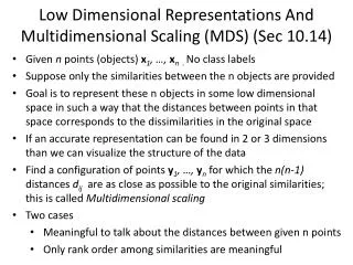
2. Multidimensional Scaling (MDS): What Is It? • Generally regarded as exploratory data analysis(Ding, 2006). • Reduces large amounts of data into easy-to-visualize structures. • Attempts to find structure (visual representation) in a set of distance measures, e.g. dis/similarities, between objects/cases. • Shows how variables/objects are related perceptually. • How? By assigning cases to specific locations in space. • Distances between points in space match dis/similarities as closely as possible: Similar objects: Close points Dissimilar objects: Far apart points

3. MDS Example: City Distances Distances Matrix: Symmetric Cluster Spatial Map Dimensions 1: North/South 2: East/West

4. The Process of MDS: The Data • Data of MDS: similarities, dissimilarities, distances, or proximities reflects amount of dis/similarity or distance between pairs of objects. • Distinction between similarity and dissimilarity data dependent on type of scale used: Dissimilarity scale: Low #=high similarity & High #=high dissimilarity. Similarity scale: Opposite of dissimilarity. • E.g. On a scale of 1-9 (1 being the same and 9 completely different) how similar are chocolate bars A and B? Dissimilarity scale. • SPSS requires dissimilarity scales.

5. Data Collection for MDS (1) • Direct/raw data: Proximities’ values directly obtained from empirical, subjective scaling. • E.g. Rating or ranking dis/similarities (Likert scales). • Indirect/derived data: Computed from other measurements: correlations or confusion data (based on mistakes) (Davidson, 1983). • E.g. Letters of alphabet presented briefly and must be identified. Rarely confused letters given high dissimilarity values, those that are confused get low values. • Data collection: Pairwise comparison, grouping/sorting tasks, direct ranking, objective method (e.g. city distances). • Pairwise comparisons: All object pairs randomly presented: # of pairs = n(n-1)/2, n = # of objects/cases Can be tedious and inefficient process.

6. Data Collection for MDS (2) Facilitation of pairwise comparison task: 1) Incomplete similarity task: random or cyclic deletion of comparison pairs. 2) Simplification of pair comparisons (binary scale). 3) Choosing grouping/sorting tasks(Tsogo et al., 2000). Pre-specified # of groups or not specified. • Appropriateness of a data collection technique is dependent on stimuli and, in some cases, “hypothesis” and theory.

7. Type of MDS Models (1) • MDS model classified according to: 1) Type of proximities: • Metric/quantitative: Quantitative information/interval data about objects’ proximities e.g. city distance. • Non-metric/qualitative: Qualitative information/nominal data about proximities e.g. rank order. 2) Number of proximity matrices (distance, dis/similarity matrix). • Proximity matrix is the input for MDS. • The above criteria yield: • 1) Classical MDS: One proximity matrix (metric or non-metric). • 2) Replicated MDS: Several matrices. • 3) WeightedMDS/IndividualDifferenceScaling: Aggregate proximities and individual differences in a common MDS space.

8. Types of MDS (2) • More typical in Social Sciences is the classification of MDS based on nature of responses: 1) Decompositional MDS: Subjects rate objects on an overall basis, an “impression,” without reference to objective attributes. • Production of a spatial configuration for an individual and a composite map for group. 2) Compositional MDS: Subjects rate objects on a variety of specific, pre-specified attributes (e.g. size). • No maps for individuals, only composite maps.

9. The MDS Model • Classical MDS uses Euclidean principles to model data proximities in geometrical space, where distance (dij) between points i and j is defined as: xi and xj specify coordinates of points i and j on dimension a, respectively. • The modeled Euclidean distances are related to the observed proximities, ij, by some transformation/function (f). • Most MDS models assume that the data have the form: ij = f(dij) • All MDS algorithms are a variation of the above (Davidson, 1983).

10. Output of MDS • MDS Map/Perceptual Map/Spatial Representation: 1) Clusters: Groupings in a MDS spatial representation. • These may represent a domain/subdomain. 2) Dimensions: Hidden structures in data. Ordered groupings that explain similarity between items. • Axes are meaningless and orientation is arbitrary. • In theory, there is no limit to the number of dimensions. • In reality, the number of dimensions that can be perceived and interpreted is limited.

11. Diagnostics of MDS (1) • MDS attempts to find a spatial configuration X such that the following is true: f(δij) ≈ dij(X) • Stress (Kruskal’s) function: Measures degree of correspondence between distances among points on the MDS map and the matrix input. Proportion of variance of disparities not accounted for by the model: • Range 0-1: Smaller stress = better representation. • None-zero stress: Some/all distances in the map are distortions of the input data. • Rule of thumb: ≤0.1 is excellent; ≥0.15 not tolerable.

12. Diagnostics of MDS (2) • R2 (RSQ): Proportion of variance of the disparities accounted for by the MDS procedure. • R2≥0.6 is an acceptable fit. • Weirdness Index: Correspondence of subject’s map and the aggregate map  outlier identification. • Range 0-1: 0 indicates that subject’s weights are proportional to the average subject’s weights; as the subject’s score becomes more extreme, index approaches 1. • Shepard Diagram: Scatterplot of input proximities (X-axis) against output distances (Y-axis) for every pair of items. • Step-line produced. If map distances fall on the step-line this indicates that input proximities are perfectly reproduced by the MDS model (dimensional solution).

13. Interpretation of Dimensions • Squeezing data into 2-D enables “readability” but may not be appropriate: Poor, distorted representation of the data (high stress). • Scree plot: Stress vs. number of dimensions. E.g. cities distance • Primary objective in dimension interpretation: Obtain best fit with the smallest number of possible dimensions. • How does one assign “meaning” to dimensions?

14. Meaning of Dimensions • Subjective Procedures: • Labelling the dimensions by visual inspection, subjective interpretation, and information from respondents. • “Experts” evaluate and identify the dimensions.

15. Validating MDS Results • Split-sample comparison: • Original sample is divided and a correlation between the variables is conducted. • Multi-sample comparison: • New sample is collected and a correlation is conducted between the old and new data. • Comparisons are done visually or with a simple correlation of coordinates or variables. Assessing whether MDS solution (dimensionality extraction) changes in a substantial way.

16. MDS Caveats • Respondents probably perceive stimuli differently. In non-aggregate data, different dimensions may emerge. • Respondents may attach different levels of importance to a dimension. • Importance of a dimension may change over time. • Interpretation of dimensions is subjective. • Generally, more than four times as many objects as dimensions should be compared for the MDS model to be stable.

17. “Advantages” of MDS • An alternative to the GLM. • Does not require assumptions of linearity, metricity, or multivariate normality. • Can be used to model nonlinear relationships. • Dimensionality “solution” can be obtained from individuals; gives insight into how individuals differ from aggregate data. • Reveals dimensions without the need for defined attributes. • Dimensions that emerge from MDS can be incorporated into regression analysis to assess their relationship with other variables.

18. “Disadvantages” of MDS • Provides a global measure of dis/similarity but does not provide much insight into subtleties (Street et al., 2001). • Increased dimensionality: Difficult to represent and decreases intuitive understanding of the data. As such, the model of the data becomes as complicated as the data itself. • Determination of meanings of dimensions is subjective.

19. A Tiny Break . . .

20. “SPSSing” MDS • In the SPSS Data Editor window, click: Analyze > Scale > Multidimensional Scaling

21. Select four or more Variables that you want to test. • You may select a single variable for the Individual Matrices for window (depending on the distances option selected).

22. If Data are distances (e.g. cities distances) option is selected, click on the Shape button to define characteristic of the dissimilarities/proximity matrices. • If Create distance from dataisselected, click on the Measure button to control the computation of dissimilarities, to transform values, and to compute distances.

23. In the Multidimensional Scaling dialog box, click on the Model button to control the level of measurement, conditionality, dimensions, and the scaling model. • Click on the Options button to control the display options, iteration criteria, and treatment of missing values.

24. MDS: A Psychological Example “Multidimensional scaling modelling approach to latent profile analysis in psychological research” (Ding, 2006) • Basic premise: Utilize MDS to investigate types or profiles of people. • “Profile:” From applied psych where test batteries are used to extract and construct distinctive features/characteristics in people. • MDS method was used to: • Derive profiles (dimensions) that could provide information regarding psychosocial adjustment patterns in adolescents. • Assess if individuals could follow different profile patterns than those extracted from group data, i.e. deviations from the derived normative profiles.

25. Study Details: Methodology • Participants: College students (µ=23 years, n=208). • Instruments: • Self-Image Questionnaire for Young Adolescents (SIQYA). Variables: • Body Image (BI), Peer Relationships (PR), Family Relationships (FR), Mastering & Coping (MC), Vocational-Educational Goals (VE), and Superior Adjustment (SA) • Three mental health measures of well-being: • Kandel Depression Scale • UCLA Loneliness Scale • Life Satisfaction Scale

26. Data for MDS • Scored data for MDS profile analysis • Sample data for 14 individuals: BI=body image, PR=peer relations, FR=family relations, MC=mastery & coping, VE=vocational & educational goal, SA=superior adjustment, PMI-1=profile match index for Profile 1, PMI-2=profile match index for Profile 2, LS=life satisfaction, Dep=depression, PL=psychological loneliness

27. The Analysis: Step by Step • Step 1: Estimate the number of profiles (dimensions) from the latent variables. • Kruskal's stress = 0.00478 • Excellent stress value. • RSQ = 0.9998 • Configuration derived in 2 dimensions.

28. Scale values of two MDS profiles (dimensions) in psychosocial adjustment. • Normative profiles of psychosocial adjustments in young adults. • Each profile represents prototypical individual.

29. Step 2: Using the estimated scale values as independent variables and observed variables as dependent variables estimate: • Individual profile match index (PMI): • The extent of individual variability along a profile. • Intra-individual variability across profiles. • Fit index: • The proportion of variance in the individual’s observed data that can be accounted for by the profiles. PMI-1=profile match index for Profile 1, PMI-2=profile match index for Profile 2, LS=life satisfaction, Dep=depression, PL=psychological loneliness

30. Individual Profiles vs. Aggregate

31. Step 3: Assess the association between profiles and other factors by regression. Profile 1: -High scores on Body Image - higher degree of life satisfaction. -High scores on the Vocational-Educational Goal - higher degree of depression. Profile 2: -Higher scores on the family relationships profile - higher degree of psychological loneliness. Level: -Average scores of individuals’ psychosocial adjustment. -Overall positive psychosocial adjustment scores suggest less depression or psychological loneliness and higher degree of life satisfaction.

32. Commentary on MDS Profile Analysis • Strength of MDS profile analysis: • Provides representation of what typical configurations or profiles of variables exist in the population and how individuals differ with respect to these profiles. • Enables identification/analysis of: • Individuals who develop in an idiographic (specific and subjective) manner; not consistent with aggregate profiles.

33. Limitations of MDS Profile Analysis • MDS profile analysis is exploratory: Determination of the number of profiles is subjective. • Because of subjectivity involved, the best methods for model selection should be based on theoretical grounds. • Interpretation of the statistical significance of the scale values (i.e. variable parameter estimates) is somewhat arbitrary. There are no objective criteria for decision-making regarding which scale values are salient. • Not know to what degree the profiles obtained from MDS can be generalized across populations.

34. Thank You! Questions?

35. References • Davidson, M. L. (1983). Multidimensional scaling. New York: J. Wiley and Sons. • Ding, C. S. (2006). Multidimensional scaling modelling approach to latent profile analysis in psychological research. International Journal of Psychology41 (3), 226-238. • Kruskal, J.B. & Wish M.1978. Multidimensional Scaling. Sage. • Street, H., Sheeran, P., & Orbell, S. (2001). Exploring the relationship between different psychosocial determinants of depression: a multidimensional scaling analysis. Journal of Affective Disorders 64,53–67. • Takane, Y., Young, F.W., & de Leeuw, J. (1977). Nonmetric individual differences multidimensional scaling: An alternating least squares method with optimal scaling features, Psychometrika42 (1), 7–67. • Young, F.W., Takane, Y., & Lewyckyj, R. (1978). Three notes on ALSCAL, Psychometrika43 (3), 433–435. • http://www.analytictech.com/borgatti/profit.htm • http://www2.chass.ncsu.edu/garson/pa765/mds.htm • http://www.terry.uga.edu/~pholmes/MARK9650/Classnotes4.pdf