Download
1 / 24
250 likes | 506 Views
Planning with Constraints Graphplan & SATplan . Yongmei Shi. Introduction. Graphplan

E N D
Planning with ConstraintsGraphplan & SATplan Yongmei Shi
Introduction • Graphplan • a general-purpose planner based on ideas used in graph algorithms. Given a problem statement, Graphplan explicitly constructs and annotates a Planning Graph, in which a plan is a kind of "flow" of truth-values through the graph. • SATplan • methods for compiling planning problems into propositional formulae for solution using systematic and stochastic SAT algorithms. • These two approaches both are impacted by constraint satisfaction and search techonology
Part I Graphplan • Graphplan alternates between two phases • graph expansion • solution extraction • graph expansion • extend a planning graph forward in "time" until it has achieved a necessary condition for plan existence • solution extraction • perform a backward-chaining search on the graph, looking for a plan that solves the problem • If no solution is found, the cycle repeats by further expanding the planning graph
Graph Expansion • The planning graph contains two types of nodes • proposition nodes • action nodes • The nodes are arranged into levels • Even-numbered levels contain proposition nodes • Odd-numbered levels correspond to action instances whose preconditions are present at previous level
Graph Expansion Cont. • Edges: • connect proposition nodes to the action instances (at the next level) whose preconditions mention those propositions • connect from action nodes to subsequent propositions made true by the action's effects • connect proposition layers, these edges represent maintenance actions that encode persistence
Graph Expansion Cont. • Binary mutual exclusion relation between nodes • Inconsistent Effect: the effect of one action is the negation of another action's effect • Interference: one action deletes the precondition of another • Competing Needs: the actions have preconditions that are mutually exclusive at level i-1 • Two propositions are mutex • if one is the negation of the other • if all ways of achieving the propositions are pairwise mutex
An example Initial Conditions: (and (garbage) (cleanHands) (quiet)) Goal: (and (dinner) (present) (not (garbage))) Actions: cook wrap carry Dolly • :precondition (cleanHands) • :effect (dinner) • :precondition (quiet) • :effect (present) :precondition :effect (and (not (garbage)) (not cleanHands))) :precondition :effect (and (not (garbage)) (not (quiet)))
0 1 2 grab grab carry ¬grab dolly cleanH cleanH ¬cleanH cook quiet quiet wrap ¬quiet {carry, cook, wrap} {dolly, cook, wrap} dinner present
0 1 2 3 4 grab grab grab carry carry ¬grab ¬grab dolly dolly cleanH cleanH cleanH ¬cleanH ¬cleanH cook cook quiet quiet quiet wrap wrap ¬quiet ¬quiet dinner dinner present present
Solution Extraction • When to perform • When planning graph has been extended to an even level i, in which all goal propositions are present and none are pairwise mutex • How to perform • consider each of the n subgoals in turn • For each literal, if more than one action produces the subgoal, it must consider all of them. If action is consistent with all actions that have been chosen so far at this level, then it proceeds to the next subgoal, otherwise it backtracks to a previous choice.
Solution Extraction Cont. • When a consistent set of actions at level i-1 is found, it try to find a plan for the set that is the union of all the preconditions of those actions at level i-2. • If all the combinations of the possible solutions are failed, the Graphplan extends the planning graph with additional action and proposition levels, then tries solution extraction again.
Optimization • Improvements for solution extraction process: • transfer many strategies from the CSP field to planning, such as: forward checking, dynamic variable ordering, memorization, and conflict-directed backjumping. • Optimizations for graph expansion process: • closed world assumption • type analysis & simplification • regression focusing • in-place graph expansion
More issues • Handling Expressive Action Language • Disjunction Precondition • Conditional Effects • Universal Quantification
Part II SATplan • Basic Idea • Compile planning problems into propositional formulae for solution using systematic and stochastic SAT algorithm
Architecture of SAT-based planning system Increment time bound if Unsatisfiable Compiler Simplifier Solver Decoder Init State Goal Actions CNF CNF SatisfyingAssignment Plan Symbol Table
Architecture of SAT-based planning system Cont. • Compiler • take a planning problem as input, guess a plan length, and generate a propositional logic formula, which if satisfied, implies the existence of a solution plan • Symbol table • record the correspondence between propositional variables and the planning instance • Simplifier • use fast techniques such as unit clause propagation and pure literal elimination to shrink the CNF formula • Solver • use systematic or stochastic methods to find a satisfying assignment. If the formula is unsatisfiable, then the compiler generates a new encoding reflecting a longer plan length • Decoder • translate the result of solver into a solution plan.
Encoding • Encoding uses the universal axioms: • INIT: the initial state is completely specified at time zero, including all properties presumed false by the closed-world assumption • garb0 ^ cleanH0 ^ quiet0 ^ ¬dinner0 ^ ¬present0 • GOAL: all desired goal properties are asserted to be true at time 2n (n is the length of plan) • ¬garb2 ^ dinner2 ^ present2 • AP,E: Action imply their preconditions and effects • (¬carry1 v dinner2) ^ (¬carry1 v cleanH0)
Encoding Cont. • Encoding is important to the performance of Solver, since solver speed can be exponential in the size of the formula. • Two dimensions need be considered • Action representation • Frame Axiom
Action representation • Specify the correspondence between propositional variables and ground plan actions • Be crucial to the parameterized action schemata • Four choices • Regular representation • Simple action split • Overload action split • Bitwise representation • The choices represent the difference of number of variables in the formula • Preliminary results suggest that the regular and simple split representations are good choices
Frame Axioms • Frame axioms constrain unaffected fluents when an action occurs • Two alternatives • Classical frame • State which fluents are left unchanged by a given action • combined with At-least-one axiom to ensure that some actions occurs at each odd time step • Explanatory frame • Enumerate the set of actions that could have occurred in order to account for a state change • combined with Exclusion axiom to enforce the constraints in the resulting plan • Experience shows that explanatory frame are clearly superior to classical frames in almost every case
SAT solvers • Systematic SAT solvers • DPLL algorithm • Perform a backtracking depth-first search through the space of partial truth assignment, using unit-clause and pure-literal heuristics • Stochastic SAT solvers • Search locally using random moves to escape from local minima. • incomplete • GSAT: perform a greedy search. After hill climbing for a fixed amount of flips, it starts anew with a freshly generated, random assignment. • WALKSAT: improve GSAT by adding additional randomness akin to simulated annealing
Procedure DPLL(CNF formula: f) If f is empty, return yes Else if there is an empty clause in f, return no Else if there is a pure literal u in f, return DPLL(f(u)) Else if there is a unit clause {u} in f, return DPLL(f(u)) Else Choose a variable v mentioned in f If DPLL(f(v)) = yes, then return yes Else return DPLL(f(!v)) Backtracking, depth-first search through the space truth assighment
Procedure GSAT(CNF formula: f, integer: Nrestart, Nflips) For I equals 1 to Nrestarts, Set A to a randomly generated truth assignment. For j equals 1 to Nflips, If A satisfies f then return yes. Else Set v to be a variable in f whose change gives the largest increase in the number of satisfied clauses; break ties randomly. Modify A by flipping the truth assignment of vRandom-restart, hill-climbing through the space of complete truth assignment
Compare Graphplan with SAT • Both approaches convert parameterized action schemata into a finite propositional structure representing the space of possible plans up to a given length • The planning graph • a CNF formula • Both approaches use local consistency methods before resorting to exhaustive search • mutex propagation • Propositional simplification • Both approaches iteratively expand their propositional structure until they find a solution • planning graph is extends when no solution is found • propositional logic formula is recreated for a longer plan length • Planning graph can be automatically converted into CNF notation for solution with SAT solvers