Download
1 / 19
190 likes | 371 Views
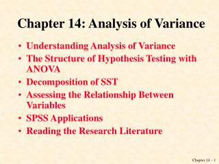
Chapter 14: Analysis of Variance. Analysis of variance is a technique that allows us to compare two or more populations. Analysis of variance is:. a procedure which determines whether differences exist between population means .

E N D
Chapter 14: Analysis of Variance Analysis of variance is a technique that allows us to compare two or more populations. Analysis of variance is:. a procedure which determines whether differences exist between population means. a procedure which works by analyzing sample means.
One-Way Analysis of Variance Independent samples are drawn from k populations: Note: These populations are referred to as treatments. It is not a requirement that n1 = n2 = … = nk.
Example 14.1 The age categories are Young (Under 35) Early middle-age (35 to 49) Late middle-age (50 to 65) Senior (Over 65) The analyst was particularly interested in determining whether the ownership of stocks varied by age. Xm14-01 Do these data allow the analyst to determine that there are differences in stock ownership between the four age groups? To help answer this question a financial analyst randomly sampled 366 American households and asked each to report the age of the head of the household and the proportion of their financial assets that are invested in the stock market.
Example 14.1 Terminology The age category is the factor we’re interested in. This is the only factor under consideration (hence the term “one way” analysis of variance). Each population is a factor level. In this example, there are four factor levels: Young, Early middle age, Late middle age, and Senior.
Example 14.1 IDENTIFY The null hypothesis in this case is: H0:µ1 = µ2 = µ3 = µ4 i.e. there are no differences between population means. Our alternative hypothesis becomes: H1: at least two means differ
Example 14.1 COMPUTE The following sample statistics and grand mean were computed
Example 14.1 COMPUTE Using Excel: Click Data, Data Analysis, Anova: Single Factor
Example 14.1 COMPUTE
Example 14.1 INTERPRET Since the p-value is .0405, which is small we reject the null hypothesis (H0:µ1 = µ2 = µ3 = µ4)in favor of the alternative hypothesis (H1: at least two population means differ). That is: there is enough evidence to infer that the mean percentages of assets invested in the stock market differ between the four age categories.
Multiple Comparisons When we conclude from the one-way analysis of variance that at least two treatment means differ (i.e. we reject the null hypothesis that H0: ), we often need to know which treatment means are responsible for these differences. We will examine two statistical inference procedures that allow us to determine which population means differ: • Fisher’s least significant difference (LSD) method • Tukey’s multiple comparison method*.
Example 14.2 North American automobile manufacturers have become more concerned with quality because of foreign competition. One aspect of quality is the cost of repairing damage caused by accidents. A manufacturer is considering several new types of bumpers. To test how well they react to low-speed collisions, 10 bumpers of each of four different types were installed on mid-size cars, which were then driven into a wall at 5 miles per hour.
Example 14.2 The cost of repairing the damage in each case was assessed. Xm14-02 a Is there sufficient evidence to infer that the bumpers differ in their reactions to low-speed collisions? b If differences exist, which bumpers differ?
Example 14.2 The cost of repairing the damage in each case was assessed. Xm14-02 14.13
Example 14.2 The problem objective is to compare four populations, the data are interval, and the samples are independent. The correct statistical method is the one-way analysis of variance. F = 4.06, p-value = .0139. There is enough evidence to infer that a difference exists between the four bumpers. The question is now, which bumpers differ?
Example 14.2 The sample means are
Example 14.2 We calculate the absolute value of the differences between means and compare them.
Example 14.2 Excel Click Add-Ins > Data Analysis Plus > Multiple Comparisons
Example 14.2 LSD Method Hence, using LSD µ1 and µ2, µ1 and µ3, µ2 and µ4, and µ3 and µ4 differ (ie. “difference” values > LSD Alpha Values) The other two pairs µ1 and µ4, and µ2 and µ3 do not differ.
Example 14.1 • Tukey’s Method Using Tukey’s method µ2 and µ4, and µ3 and µ4 differ. (ie. “difference” values > Omega Alpha Values)