Download
1 / 31
340 likes | 574 Views
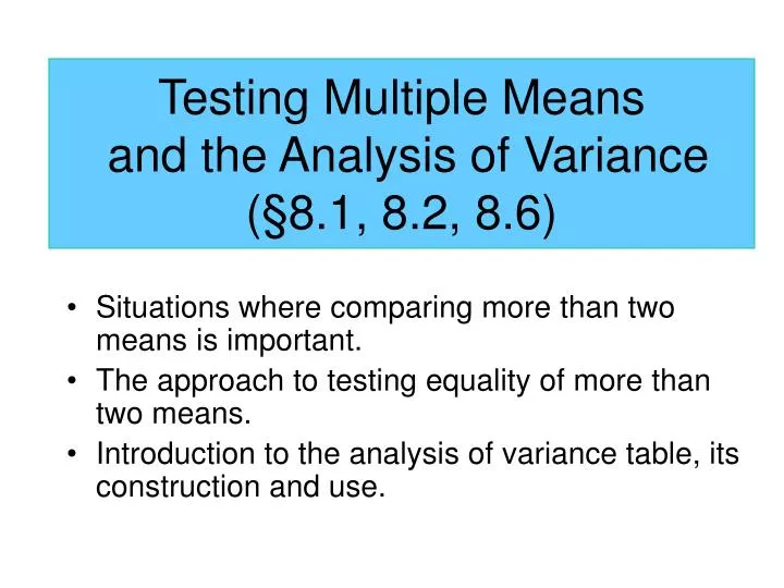
Testing Multiple Means and the Analysis of Variance ( §8.1, 8.2, 8.6 ). Situations where comparing more than two means is important. The approach to testing equality of more than two means. Introduction to the analysis of variance table, its construction and use.

E N D
Testing Multiple Means and the Analysis of Variance (§8.1, 8.2, 8.6) • Situations where comparing more than two means is important. • The approach to testing equality of more than two means. • Introduction to the analysis of variance table, its construction and use.
Simple Random Sample from a population with known s - continuous response. Simple Random Sample from a population with unknown s - continuous response. Simple RandomSamples from 2 popns with known s. Simple Random Samples from 2 popns with unknown s. One sample z-test. One sample t-test. Two sample z-test. Two sample t-test. Study Designs and Analysis Approaches
Sampling Study with t>2 Populations One sample is drawn independently and randomly from each of t > 2 populations. Objective: to compare the means of the t populations for statistically significant differences in responses. Initially we will assume all populations have common variance, later, we will test to see if this is indeed true. (Homogeneity of variance tests).
Sampling Study Vegetarians Meat & Potato Eaters Health Eaters Random Sample Random Sample Random Sample Cholesterol Levels
Experimental Studywith t>2 treatments Experimental Units: samples of size n1, n2, …, nt, are independently and randomly drawn from each of the t populations. Separate treatmentsare applied to each sample. A treatment is something done to the experimental units which would be expected to change the distribution (usually only the mean) of the response(s). Note: if all samples are drawn from the same population before application of treatments, the homogeneity of variances assumption might be plausible.
Cholesterol Levels @ 1 year. Experimental Study Male College Undergraduate Students Veg. Diet Health Diet Random Sampling M & P Diet Set of Experimental Units Set of Experimental Units Set of Experimental Units Responses
Hypothesis Let mi be the true mean of treatment group i (or population i ). Hence we are interested in whether all the groups (populations) have exactly the same true means. The alternative is that some of the groups (populations) differ from the others in their means. Let 0be the hypothesized common mean under H0.
A Simple Model Let yij be the response for experimental unit j in group i, i=1,2, ..., t, j=1,2, ..., ni. The model is: E(yij)= i: we expect the group mean to be mi. eij is the residual or deviation from the group mean. Each population has normally distributed responses around their own means, but the variances are the same across all populations. Assuming yij ~ N(mi, s2), then eij ~ N(0, s2) If H0 holds, yij = m0 + eij , that is, all groups have the same mean and variance.
A Naïve Testing Approach Test each possible pair of groups by performing all pair-wise t-tests. • Assume each test is performed at the a=0.05 level. • For each test, the probability of not rejecting Ho when Ho is true is 0.95 (1-a). • The probability of not rejecting Ho when Ho is true for all three tests is (0.95)3 = 0.857. • Thus the true significance level (type I error) for the overall test of no difference in the means will be 1-0.857 = 0.143, NOT the a=0.05 level we thought it would be. Also, in each individual t-test, only part of the information available to estimate the underlying variance is actually used. This is inefficient - WE CAN DO MUCH BETTER!
Within groups variance Between sample means variance Testing Approaches - Analysis of Variance The term “analysis of variance” comes from the fact that this approach compares the variability observed between sample means to a (pooled) estimate of the variability among observations within each group (treatment).
Within group variance is small compared to variability between means. Clear separation of means. Within group variance is large compared to variability between means. Unclear separation of means. Extreme Situations
Extend the concept of a pooled variance to t groups as follows: If all the ni are equal to n then this reduces to an average variance. Pooled Variance From two-sample t-test with assumed equal variance, s2, we produced a pooled (within-group) sample variance estimate.
Variance Between Group Means Consider the variance between the group means computed as: If we assume each group is of the same size, say n, then under H0, s2 is an estimate of s2/n (the variance of the sampling distribution of the sample mean). Hence, n times s2 is an estimate of s2. When the sample sizes are unequal, the estimate is given by: where
F-test Now we have two estimates of s2, within and between means. An F-test can be used to determine if the two statistics are equal. Note that if the groups truly have different means, sB2 will be greater than sw2. Hence the F-statistic is written as: If H0 holds, the computed F-statistics should be close to 1. If HA holds, the computed F-statistic should be much greater than 1. We use the appropriate critical value from the F - table to help make this decision. Hence, the F-test is really a test of equality of means under the assumption of normal populations and homogeneous variances.
Partition of Sums of Squares SSB SSW = + TSS Total Sums of Squares Sums of Squares Between Means Sums of Squares Within Groups + = TSS measures variability about the overall mean
Partition of the sums of squares Partition of the degrees of freedom Test Statistic Variance Estimates The AOV (Analysis of Variance) Table The computations needed to perform the F-test for equality of variances are organized into a table.
Example-Excel =average(b6:b10) =var(b6:b10) =sqrt(b13) =count(b6:b10) =(B15-1)*B13 =(sum(B15:D15)-1)*var(B6:D10) =sum(b16:d16) =b18-b19
Example SAS proc anova; class popn; model resp = popn ; title 'Table 13.1 in Ott - Analysis of Variance'; run; Table 13.1 in Ott - Analysis of Variance 31 Analysis of Variance Procedure Dependent Variable: RESP Sum of Mean Source DF Squares Square F Value Pr > F Model 2 2.03333333 1.01666667 5545.45 0.0001 Error 12 0.00220000 0.00018333 Corrected Total 14 2.03553333 R-Square C.V. Root MSE RESP Mean 0.998919 0.247684 0.013540 5.466667 Source DF Anova SS Mean Square F Value Pr > F POPN 2 2.03333333 1.01666667 5545.45 0.0001
GLM in SAS General Linear Models Procedure Dependent Variable: RESP Sum of Mean Source DF Squares Square F Value Pr > F Model 2 2.03333333 1.01666667 5545.45 0.0001 Error 12 0.00220000 0.00018333 Corrected Total 14 2.03553333 R-Square C.V. Root MSE RESP Mean 0.998919 0.247684 0.013540 5.466667 Source DF Type I SS Mean Square F Value Pr > F POPN 2 2.03333333 1.01666667 5545.45 0.0001 Source DF Type III SS Mean Square F Value Pr > F POPN 2 2.03333333 1.01666667 5545.45 0.0001 T for H0: Pr > |T| Std Error of Parameter Estimate Parameter=0 Estimate INTERCEPT 5.000000000 B 825.72 0.0001 0.00605530 POPN 1 0.900000000 B 105.10 0.0001 0.00856349 2 0.500000000 B 58.39 0.0001 0.00856349 3 0.000000000 B . . . NOTE: The X'X matrix has been found to be singular and a generalized inverse was used to solve the normal equations. Estimates followed by the letter 'B' are biased, and are not unique estimators of the parameters. proc glm; class popn; model resp = popn / solution; title 'Table 13.1 in Ott’; run;
Minitab Example STAT > ANOVA > OneWay (Unstacked) One-way Analysis of Variance Analysis of Variance Source DF SS MS F P Factor 2 2.033333 1.016667 5545.45 0.000 Error 12 0.002200 0.000183 Total 14 2.035533 Individual 95% CIs For Mean Based on Pooled StDev Level N Mean StDev ----+---------+---------+---------+-- EG1 5 5.9000 0.0158 (* EG2 5 5.5000 0.0071 *) EG3 5 5.0000 0.0158 (* ----+---------+---------+---------+-- Pooled StDev = 0.0135 5.10 5.40 5.70 6.00
Function: lm( ) R Example > hwages <- c(5.90,5.92,5.91,5.89,5.88,5.51,5.50,5.50,5.49,5.50,5.01, 5.00,4.99,4.98,5.02) > egroup <- factor(c(1,1,1,1,1,2,2,2,2,2,3,3,3,3,3)) > wages.fit <- lm(hwages~egroup) > anova(wages.fit) Df Sum Sq Mean Sq F value Pr(>F) factor(egroup) 2 2.03333 1.01667 5545.5 2.2e-16 *** Residuals 12 0.00220 0.00018 --- Signif. codes: 0 `***' 0.001 `**' 0.01 `*' 0.05 `.' 0.1 ` ' 1
> summary(wages.fit) R Example Call: lm(formula = hwages ~ egroup) Residuals: Min 1Q Median 3Q Max -2.000e-02 -1.000e-02 -1.941e-18 1.000e-02 2.000e-02 Coefficients: Estimate Std. Error t value Pr(>|t|) (Intercept) 5.900000 0.006055 974.35 < 2e-16 *** egroup2 -0.400000 0.008563 -46.71 6.06e-15 *** egroup3 -0.900000 0.008563 -105.10 < 2e-16 *** --- Signif. codes: 0 '***' 0.001 '**' 0.01 '*' 0.05 '.' 0.1 ' ' 1 Residual standard error: 0.01354 on 12 degrees of freedom Multiple R-Squared: 0.9989, Adjusted R-squared: 0.9987 F-statistic: 5545 on 2 and 12 DF, p-value: < 2.2e-16 (Intercept) egroup2 egroup3 5.9 -0.4 -0.9
A Nonparametric Alternative to the AOV Test: The Kruskal - Wallis Test (§8.5) What can we do if the normality assumption is rejected in the one-way AOV test? We can use the standard nonparametric alternative: the Kruskal-Wallis Test. This is an extension of the Wilcoxon Rank Sum Test to more than two samples. .
Kruskal - Wallis Test Extension of the rank-sum test for t=2 to the t>2 case. H0: The center of the t groups are identical. Ha: Not all centers are the same. Test Statistic: Ti denotes the sum of the ranks for the measurements in sample i after the combined sample measurements have been ranked. Reject if H > c2(t-1),a With large numbers of ties in the ranks of the sample measurements use: where tj is the number of observations in the jth group of tied ranks.
OBS POPN RESP 1 1 5.90 2 1 5.92 3 1 5.91 4 1 5.89 5 1 5.88 6 2 5.51 7 2 5.50 8 2 5.50 9 2 5.49 10 2 5.50 11 3 5.01 12 3 5.00 13 3 4.99 14 3 4.98 15 3 5.02 options ls=78 ps=49 nodate; data OneWay; input popn resp @@ ; cards; 1 5.90 1 5.92 1 5.91 1 5.89 1 5.88 2 5.51 2 5.50 2 5.50 2 5.49 2 5.50 3 5.01 3 5.00 3 4.99 3 4.98 3 5.02 ; run; proc print; run; Proc npar1way; class popn; var resp; run;
Analysis of Variance for Variable resp Classified by Variable popn popn N Mean ƒƒƒƒƒƒƒƒƒƒƒƒƒƒƒƒƒƒƒƒƒƒƒƒƒƒƒƒƒƒƒƒƒƒƒƒƒƒ 1 5 5.90 2 5 5.50 3 5 5.00 Source DF Sum of Squares Mean Square F Value Pr > F ƒƒƒƒƒƒƒƒƒƒƒƒƒƒƒƒƒƒƒƒƒƒƒƒƒƒƒƒƒƒƒƒƒƒƒƒƒƒƒƒƒƒƒƒƒƒƒƒƒƒƒƒƒƒƒƒƒƒƒƒƒƒƒƒƒƒƒ Among 2 2.033333 1.016667 5545.455 <.0001 Within 12 0.002200 0.000183 Average scores were used for ties.
The NPAR1WAY Procedure Wilcoxon Scores (Rank Sums) for Variable resp Classified by Variable popn Sum of Expected Std Dev Mean popn N Scores Under H0 Under H0 Score ƒƒƒƒƒƒƒƒƒƒƒƒƒƒƒƒƒƒƒƒƒƒƒƒƒƒƒƒƒƒƒƒƒƒƒƒƒƒƒƒƒƒƒƒƒƒƒƒƒƒƒƒƒƒƒƒƒƒƒƒƒƒƒƒƒƒƒƒ 1 5 65.0 40.0 8.135753 13.0 2 5 40.0 40.0 8.135753 8.0 3 5 15.0 40.0 8.135753 3.0 Average scores were used for ties. Kruskal-Wallis Test Chi-Square 12.5899 DF 2 Pr > Chi-Square 0.0018
MINITAB Stat > Nonparametrics > Kruskal-Wallis Kruskal-Wallis Test: RESP versus POPN Kruskal-Wallis Test on RESP POPN N Median Ave Rank Z 1 5 5.900 13.0 3.06 2 5 5.500 8.0 0.00 3 5 5.000 3.0 -3.06 Overall 15 8.0 H = 12.50 DF = 2 P = 0.002 H = 12.59 DF = 2 P = 0.002 (adjusted for ties)
R kruskal.test( ) > kruskal.test(hwages,factor(egroup)) Kruskal-Wallis rank sum test data: hwages and factor(egroup) Kruskal-Wallis chi-squared = 12.5899, df = 2, p-value = 0.001846