Download
1 / 55
550 likes | 704 Views
Graphing Descriptions of Data Variables. Notes 22 - Sections 14.1-14.2. Data Set. A data set is a collection of data values. Statisticians refer to the individual data values in a data set as data points . Use the letter N to represent the size of the data set. Data Set.

E N D
Graphing Descriptions of Data Variables Notes 22 - Sections 14.1-14.2
Data Set • A data set is a collection of data values. • Statisticians refer to the individualdata values in a data set as data points. • Use the letter N to represent the size of the data set.
Data Set • Data sets can range in size from reasonably small (a dozen or sodata points) to very large (hundreds of millions of data points). • The larger thedata set is, the more we need a good way to describe and summarize it.
Example – Stat 101 Test Scores The day after the midterm exam in his Stat 101 class, Dr. Blackbeard hasposted the results online. The data set consists of N = 75data points(the number of students who took the test). Each data point (listed in the secondcolumn) is a score between 0 and 25 (Dr. Blackbeard does not give partial credit). The numbers listed in the first column are not data points – they arenumerical IDs used as substitutes for names to protect the students’ rights ofprivacy.
Example – Stat 101 Test Scores The students in the Stat 101 class want to know: How did I do? Eachstudent can answer this question directly from the table. How did the class as a whole do?
Example – Stat 101 Test Scores: Part 2 The first step is summarizing the information in Table 14-1 is to organize thescores in a frequency table such as Table 14-2. In this table, the number beloweach score gives the frequency of the score – the number of students gettingthat particular score.
Example – Stat 101 Test Scores: Part 2 Looking at Table 14-2, there was onestudent with a score of 1, one with a score of 6, two with a score of 7, six with ascore of 8, and so on. Notice that the scores with a frequency of zero are not listedin the table.
Example – Stat 101 Test Scores: Part 2 Figure 14-1 (next slide) shows the same information in a much more visual waycalled a bar graph - the test scores listed in increasing order on a horizontalaxis and the frequency of each test score displayed by the heightof the columnabove that test score. In the bar graph, even the test scores with afrequency of zero show up – there simply is no column above these scores.
Example – Stat 101 Test Scores: Part 2 Figure 14-1
Example – Stat 101 Test Scores: Part 2 Bar graphs are easy to read, and they are a nice way to present a good general picture of the data. With a bar graph, for example, it is easy to detectoutliers - extreme data points that do not fit into the overall pattern of thedata. In this example there are two obvious outliers – the score of 24 (head andshoulders above the rest of the class) and the score of 1 (lagging way behindthe pack).
Example – Stat 101 Test Scores: Part 2 Sometimes it is more convenient to express the bar graph in terms ofrelative frequencies – that is, the frequencies given in terms of percentages ofthe total population. Figure 14-2 shows a relative frequency bar graph for theStat 101 data set. Notice that we are dealingwith percentages rather than total counts and that the size of the data set is N = 75.
Example – Stat 101 Test Scores: Part 2 Figure 14-2
Example – Stat 101 Test Scores: Part 2 This allows anyone to compute the actual frequencies. For example,Fig. 14-2 indicates that 12% of the75 students scored a 12 on theexam, so the actual frequency isgiven by 75 0.12 = 9students. The change from actual frequencies to percentages (or vice versa)does not change the shape of thegraph – it is basically a change ofscale.
Bar Graph versus Pictogram Frequency charts that use iconsor pictures instead of bars to showthe frequencies are commonly referred to as pictograms. The point ofa pictogram is that a graph is oftenused not only to inform but also toimpress and persuade, and, in suchcases, a well-chosen icon or picturecan be a more effective tool thanjust a bar. Here’s a pictogram displaying the same data as in figure 14-2.
Bar Graph versus Pictogram Figure 14-3
Example – Selling the XYZ Corporation This figure is a pictogram showing the growth in yearly sales of theXYZ Corporation between 2001 and 2006. It’s a good picture to show at a shareholders meeting,but the picture is actually quite misleading.
Example – Selling the XYZ Corporation This figure shows apictogram for exactlythe same data with amuch more accurateand sobering picture ofhow well the XYZ Corporation had been doing.
Example – Selling the XYZ Corporation The difference between the two pictograms can be attributed to a coupleof standard tricks of the trade: (1) stretching the scale of the vertical axis and (2) “cheating” on the choice of starting value on the vertical axis. As an educatedconsumer, you should always be on the lookout for these tricks. In graphicaldescriptions of data, a fine line separates objectivity from propaganda.
Variable Before we continue with our discussion of graphs, we need to discuss briefly theconcept of a variable. In statistical usage, a variable is any characteristic that varieswith the members of a population. The students in Dr. Blackbeard’s Stat 101 course(the population) did not all perform equally on the exam.
Variable Thus, the test score is avariable, which in this particular case is a whole number between 0 and 25. In someinstances, such as when the instructor gives partial credit, a test score may take on a fractional value, such as 18.5 or 18.25. Evenin these cases, however, the possible increments for the values of the variable aregiven by some minimum amount – a quarter-point, a half-point, whatever.
Variable In contrast to this situation, consider a different variable: the amount of time each studentstudied for the exam. In this case the variable can take on values that differ by anyamount: an hour, a minute, a second, a tenth of a second, and so on.
Numerical Variable A variable that represents a measurable quantity is called a numerical(or quantitative) variable. When the difference between the values of a numerical variable can be arbitrarily small, we call the variable continuous (person’s height, weight, foot size, time it takes to run one mile). When possible values of the numerical variable change by minimum increments,the variable is called discrete (person’s IQ, SAT score, shoe size, score of a basketball game).
Categorical Variable Variables can also describe characteristics that cannot be measured numerically: nationality, gender, hair color, and so on. Variables of this type are calledcategorical (or qualitative) variables.
Categorical Variable In some ways, categorical variables must be treated differently from numericalvariables – they cannot, for example, be added, multiplied, or averaged. In other ways,categorical variables can be treated much like discrete numerical variables, particularly when it comes to graphical descriptions, such as bar graphs and pictograms.
Example – Enrollments at Tasmania State University Table 14-3 shows undergraduate enrollments in each of the five schools at TasmaniaState University. A sixth category (“other”) includes undeclared students, interdisciplinary majors, and so on.
Example – Enrollments at Tasmania State University Vertical and horizontal bar graphs displaying the data for Table 14-3.
Example – Enrollments at Tasmania State University When the number of categories is small, another common way to describethe relative frequencies of the categories is by using a pie chart. In apie chart the “pie” represents the entire population (100%), and the “slices” represent the categories (or classes), with the size (angle) of each slice being proportionalto the relative frequency of the corresponding category.
Example – Enrollments at Tasmania State University Some relative frequencies, such as 50% and 25%, are very easy to sketch, buthow do we accurately draw the slice corresponding to a more complicated frequency,say, 32.47%?
Example – Enrollments at Tasmania State University Here, a little elementary geometry comes in handy.Since 100%equals 360º, 1% corresponds to an angle of 360º/100 = 3.6º. Thus the frequency 32.47% is given by 32.47 3.6º = 117º (rounded to the nearest degree,which is generally good enough for most practical purposes).
Example – Enrollments at Tasmania State University This figure shows anaccurate pie chart for the school-enrollmentdata given inTable 14-3.
PIE CHARTS The general rule in drawing pie charts is that a slice representing x% is givenby an angle of (3.6)x degrees.
Example – Who’s Watching the Boob Tube Tonight? According to Nielsen Media Research data, the percentages of the TV audiencewatching TV during prime time (8 P.M. to 11 P.M.), broken up by age group, are asfollows: adults (18 years and older): 63% teenagers (12–17 years) 17% children(2–11 years) 20%
Example – Who’s Watching the Boob Tube Tonight? The pie chart shows this breakdown of audience composition by age group. A pie chart such as this one might be used to make the point thatchildren and teenagers really do not watch as much TV as it is generally believed.
Example – Who’s Watching the Boob Tube Tonight? The problem with this conclusion is that children make up only 15% of the population at large and teens only 8%. In relative terms, a higher percentage ofteenagers (taken out of the total teenage population) watch prime-time TV thanany other group, with children second and adults last.
Example – Who’s Watching the Boob Tube Tonight? Using absolute percentages can be quite misleading. When comparing characteristics of a populationthat is broken up into categories, it is essential to take into account the relativesizes of the various categories.
How Many Categories When it comes to deciding how best to display graphically the frequencies of a population, a critical issue is the number of categoriesinto which the data can fall.
How Many Categories When the number of categories is too big (say, in thedozens), a bar graph or pictogram can become muddled andineffective. This happens more often than not with numericaldata – numerical variables can take on infinitely many values, andeven when they don’t, the number of values can be too large for anyreasonable graph.
Example – 2007 SAT Math Scores The college dreams and aspirations of millions of high school seniorsoften ride on their SAT scores. The SAT consists of three sections: amath section, a writing section, and a critical reading section, withthe scores for each section ranging from a minimum of 200 to a maximum of 800 and going up in increments of 10 points. In 2007, there were 1,494,531 college-bound seniors who tookthe SAT. How do we describe the math section results for thisgroup of students?
Example – 2007 SAT Math Scores We couldset up a frequency table (or a bar graph) with the number of students scoring each of the possible scores – 200, 210, 220, 790,800. The problem is that there are 61 different possible scores between 200 and 800, and this number is too large for an effectivebar graph.
Example – 2007 SAT Math Scores In situations such as this one it is customary to present a morecompact picture of the data by grouping together, or aggregating,sets of scores into categories called class intervals. The decision as to how the class intervals are defined and how many there arewill depend on how much or how little detailis desired, but as a general rule of thumb, thenumber of class intervals should be somewhere between 5 and 20.
Example – 2007 SAT Math Scores SAT scores are usually aggregated into 12 class intervals of essentially the samesize: 200–249 250–299 300–349 700–749 750–800
Example – 2007 SAT Math Scores Here is the associated bar graph.
Example – Stat 101 Test Scores: Part 3 The process of converting test scores (a numericalvariable) into grades (acategoricalvariable) requires setting up class intervalsfor the various lettergrades. Typically, the professor has thelatitude to decide how to do this. One standard approach is to use an absolutegrading scale, usually with class intervalsof (almost) equal length for all gradesexcept F. (e.g., A = 90-100%, B = 80-89%, C = 70-79%, D = 60-69%, F = 0-59%).
Example – Stat 101 Test Scores: Part 3 Another frequently usedapproach is to use a relative grading scale. The professor fits the class intervals for the grades to the performance ofthe class in the test, often using class intervals of varying lengths. Some peoplecall this “grading on the curve,” although this terminology is somewhat misused. To illustrate relative grading in action, let’s revisit the Stat 101 midtermscores discussed in Example 14.1.
Example – Stat 101 Test Scores: Part 3 After looking at the overall class performance,Dr. Blackbeard chooses to “curve” the test scores usingclass intervals of his own creation.
Example – Stat 101 Test Scores: Part 3 The grade distribution in the Stat 101 midterm can now be best seen bymeans of a bar graph. The picture speaks for itself – thiswas a very tough exam!
Capture-Recapture Method When a numerical variable is continuous, its possible values can vary by infinitesimally small increments. As a consequence, there are no gaps between the classintervals, and our old way of doing things (using separated columns or stacks) willno longer work. In this case we use a variation of a bar graph called a histogram.
Example – Starting Salaries of TSU Graduates Suppose we want to use a graph to display the distribution of starting salaries for last year’s graduating class at Tasmania State University. The starting salaries of the N = 3258 graduates range from a low of $40,350 to a high of$74,800. Based on this range and the amount ofdetail we want to show, we must decide on thelength of the class intervals. A reasonable choicewould be to use class intervals defined in increments of $5000.
Example – Starting Salaries of TSU Graduates