Download
1 / 58
680 likes | 1.04k Views
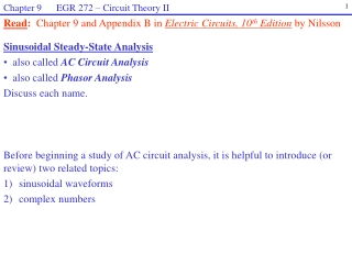
Chapter 9 EGR 272 – Circuit Theory II. 1. Read : Chapter 9 and Appendix B in Electric Circuits, 10 th Edition by Nilsson. Sinusoidal Steady-State Analysis also called AC Circuit Analysis also called Phasor Analysis Discuss each name.

E N D
Chapter 9 EGR 272 – Circuit Theory II 1 Read: Chapter 9 and Appendix B in Electric Circuits, 10th Edition by Nilsson • Sinusoidal Steady-State Analysis • also called AC Circuit Analysis • also called Phasor Analysis • Discuss each name. • Before beginning a study of AC circuit analysis, it is helpful to introduce (or review) two related topics: • 1) sinusoidal waveforms • 2) complex numbers
Chapter 9 EGR 272 – Circuit Theory II 2 Sinusoidal Waveforms In general, a sinusoidal voltage waveform can be expressed as: v(t) = Vpcos(wt) where Vp = peak or maximum voltage w = radian frequency (in rad/s) T = period (in seconds) f = frequency in Hertz (Hz) Example: An AC wall outlet has VRMS = 120V and f = 60 Hz. Express the voltage as a time function and sketch the voltage waveform.
Chapter 9 EGR 272 – Circuit Theory II 3 • Shifted waveforms: • v(t) = Vpcos(wt + ) where = phase angle in degrees • a shift to the left is positive and a shift to the right is negative (as with any function) Example: Sketch v(t) = 50cos(500t – 30o) Radians versus degrees: Note that the argument of the cosine in v(t) = Vpcos(wt + ) has mixed units – both radians and degrees. If this function is evaluated at a particular time t, care must be taken such that the units agree. Example: Evaluate v(t) = 50cos(500t – 40o) at t = 1ms.
Chapter 9 EGR 272 – Circuit Theory II 4 Relative shift between waveforms: V1 leads V2 by or V2 lags V1 by • Example: v1(t) = 50cos(500t – 50o) and v2(t) = 40cos(500t + 60o). • Does v1 lead or lag v2? By how much? • If v1 was shifted 0.5ms to the right, find a new expression for v1(t).
Chapter 9 EGR 272 – Circuit Theory II 5 • Complex Numbers • A complex number can be expressed in two forms: • Rectangular form • Polar form • A complex number can be plotted on the complex plane, where • x-axis: real part of the complex number • y-axis: imaginary (j) part of the complex number
Chapter 9 EGR 272 – Circuit Theory II 6 Rectangular Numbers A rectangular number specifies the x,y location of complex number in the complex plane in the form: (rectangular form)
Chapter 9 EGR 272 – Circuit Theory II 7 Polar Numbers A polar number specifies the distance and angle of complex number from the origin in the complex plane in the form:
Chapter 9 EGR 272 – Circuit Theory II 8 • Converting between rectangular form and polar form • Polar to Rectangular:Rectangular to Polar: • Given: |X|, Given: A, B • Find: A, B Find: |X|, A = |X|cos() B = |X|sin()
Chapter 9 EGR 272 – Circuit Theory II 9 Complex numbers using calculators Refer to the handout entitled “Complex Numbers” Mathematical Operations Using Complex Numbers Note: Calculators are used for most numerical calculations. When symbolic calculations are used, the following items may be helpful. 1) Addition/Subtraction – easiest in rectangular form
Chapter 9 EGR 272 – Circuit Theory II 10 2) Multiplication/Division – easiest in polar form 3) Inversion
Chapter 9 EGR 272 – Circuit Theory II 11 4) Exponentiation 5) Conjugate Example:
Chapter 9 EGR 272 – Circuit Theory II 12 Example: Convert to the other form or simplify. 1) -3 2) -j3 3) j6 4) -4/j 5) 1/(j2) 6) j2 7) j3 8) j4 9) 300 – j250 10) 250-75° 11) (-3 - j6)* 12) (250-75°)* 13) (4 + j7)2 14) (-4 + j6)-1
Chapter 9 EGR 272 – Circuit Theory II 13 Example: Simplify the following (by hand or using a calculator) • Note for Mastering Engineering: • If a problem asks you to enter a result as a “complex number”, use rectangular form. • If a problem asks you to enter a result in “polar form”, use polar form.
Chapter 9 EGR 272 – Circuit Theory II 14 Phasor Analysis “I have found the equation that will enable us to transmit electricity through alternating current over thousands of miles. I have reduced it to a simple problem in algebra.” Charles Proteus Steinmetz The use of complex numbers to solve ac circuit problems – the so-called phasor method considered in this chapter – was first done by German-Austrian mathematician and electrical engineer Charles Proteus Steinmetz in a paper presented in 1893. He is noted also for the laws of hysteresis and for his work in manufactured lighting. Steinmetz was born in Breslau, Germany, the son of a government railway worker. He was deformed from birth and lost his mother when he was 1 year old, but this did not keep him from becoming a scientific genius. Just as his work on hysteresis later attracted the attention of the scientific community, his political activities while he was at the University at Breslau attracted the police. He was forced to flee the country just as he had finished the work for his doctorate, which he never received. He did electrical research in the United States, primarily with the General Electric Company. His paper on complex numbers revolutionized the analysis of ac circuits, although it was said at the time that no one but Steinmetz understood the method. In 1897 he also published the first book to reduce ac calculations to a science. (Electric Circuit Analysis, 2nd Edition, by Johnson, Johnson, and Hilburn, p. 307)
Chapter 9 EGR 272 – Circuit Theory II 15 Phasor– a complex number in polar form representing either a sinusoidal voltage or a sinusoidal current. Symbolically, if a time waveform is designated at v(t), then the corresponding phasor is designated by . Examples: Convert to the other notation (time waveform or phasor) • Should phasors use cos( ) or sin( )? • It doesn’t matter as long as you are consistent. • Our textbook typically uses cos( ).
Chapter 9 EGR 272 – Circuit Theory II 16 Justification for “phasor analysis” Consider the circuit shown below. v1(t) and v2(t) must have the same form as the voltage source, v(t) (or forcing function). So v1(t) = V1cos(wt+) and v2(t) =V2cos(wt+) KVL yields: v(t) = v1(t) + v2(t) (KVL in the time-domain) VPcos(wt+) = V1cos(wt+) + V2cos(wt+) Now replacing the equation by an equation with the same real part: VPej(wt+) = V1ej(wt+) + V2ej(wt+) Dividing by ejwt yields VPej = V1ej + V2ej But these are simply polar numbers (in true polar form) so VP = V1 + V2 or (KVL using phasors) This is essentially a short proof showing why phasor analysis works.
Chapter 9 EGR 272 – Circuit Theory II 17 Before we get into the details of phasor analysis, we need a method of representing components in AC circuits. We will introduce a new term called impedance. Complex Impedance Z = impedance or complex impedance (in ) Note that the relationship above is similar to Ohm’s Law. Now we will define impedance for resistors, inductors, and capacitors. Resistors: If i(t) = Ipcos(wt + ), find v(t) and show that
Chapter 9 EGR 272 – Circuit Theory II 18 Inductors: If i(t) = Ipcos(wt + ), find v(t) and show that Capacitors: If v(t) = Vpcos(wt + ), find i(t) and show that
Chapter 9 EGR 272 – Circuit Theory II 19 AC Circuit Analysis Procedure: 1) Draw the phasor circuit (showing voltage and current sources as phasors and using complex impedances for the components). 2) Analyze the circuit in the same way that you might analyze a DC circuit. 3) Convert the final phasor result back to the time domain. Example: Find I(t) in the circuit below using phasor analysis.
Chapter 9 EGR 272 – Circuit Theory II 20 KVL and KCL in AC circuits: KVL and KCL are satisfied in AC circuits using phasor voltages and currents. They are not satisfied using the magnitudes of the voltages or the currents. Example: For the previous example, show that: Example: For the previous example, show that using a phasor diagram.
Chapter 9 EGR 272 – Circuit Theory II 21 Example: Analyze the circuit below using phasor analysis. Specifically, A) Find the total circuit impedance B) Find the total current, i(t) (Example is continued on the following slide)
Chapter 9 EGR 272 – Circuit Theory II 22 Example: (continued) C) Use current division to find i1(t) and i2(t) Show that KCL is satisfied using current phasors, but not current magnitudes. E) Show that KCL is satisfied using a phasor diagram.
Chapter 9 EGR 272 – Circuit Theory II 23 _ V2 + + + V1 V3 _ _ _ + V4 Using Phasors to Add Sinusoids Sinusoidal voltages or currents could be added using various trigonometric identities; however, they are more easily combined using phasors. Example: If v1 = 10cos(200t + 15), v2 = 15cos(200t + -30), and v3 = 8sin(200t), find v4.
Chapter 9 EGR 272 – Circuit Theory II 24 • Review of DC Circuit Analysis Techniques • Analyzing AC circuits is very similar to analyzing DC resistive circuits. Several examples are presented below which will also serve to review many DC analysis techniques, including: • Source transformations • Mesh equations • Node equations • Superposition • Operational Amplifiers (op amps) • Thevenin’s and Norton’s theorems • Maximum Power Transfer theorem
Chapter 9 EGR 272 – Circuit Theory II 25 • Source transformations • A phasor voltage source with a series impedance may be transformed into a phasor current source with a parallel impedance as illustrated below. The two sources are identical as far as the load is concerned. • Notes: • Not all sources can be transformed. Discuss. • The two sources are not equivalent internally. For example, the voltage across Zs is not equivalent to the voltage across Zp. • Dependent sources can be transformed. Converting a real current source to a real voltage source: Converting a real voltage source to a real current source:
Chapter 9 EGR 272 – Circuit Theory II 26 Example: Solve for the voltage V using source transformations.
Chapter 9 EGR 272 – Circuit Theory II 27 Mesh equations: Example: Solve for the voltage V using mesh equations.
Chapter 9 EGR 272 – Circuit Theory II 28 Node equations: Example: Solve for the current i(t) using node equations.
Chapter 9 EGR 272 – Circuit Theory II 29 • Superposition: • Superposition can be used to analyze multiple-source AC circuits in a manner very similar to analyzing DC circuits. However, there are two special cases where it is highly recommended that superposition be used: • Circuits that include sources at two or more different frequencies. • Circuits that include both DC and AC sources (Note: you could think of DC • sources as acting like AC sources with w = 0.) Example 1 (sources with different frequencies): Solve for the voltage V using superposition.
Chapter 9 EGR 272 – Circuit Theory II 30 Example 2 (AC and DC sources): Solve for the voltage V using superposition.
Chapter 9 EGR 272 – Circuit Theory II 31 • Thevenin’s and Norton’s Theorems – Recall that any one-port network N may be represented by either of the following types of equivalent circuits: • Thevenin Equivalent Circuit (TEC) – consisting of a voltage source and a series impedance • Norton Equivalent Circuit (NEC) – consisting of a current source and a parallel impedance I I I Network N independent sources, dependent sources, and resistors Network N (independent sources, dependent sources, and resistors) + V _ + V _ + V _ RTH RN + - IN VTH Load Load Load NEC TEC where:
Chapter 9 EGR 272 – Circuit Theory II 32 Thevenin’s and Norton’s Theorems with AC Circuits: Thevenin’s and Norton’s theorems apply to AC circuits as well, but and are now phasors and RTH or RN are replaced by ZTH or ZN as shown below. Network N (independent sources, dependent sources, resistors, capacitors, & inductors) I I I Network N independent sources, dependent sources, and resistors + V _ + V _ + V _ ZTH ZN + - IN VTH Load Load Load NEC TEC where:
Chapter 9 EGR 272 – Circuit Theory II 33 Thevenin’s Theorem: Example: Find the Thevenin Equivalent Circuit seen by RL in the circuit below. + _ 3mH 30 RL 50cos(5000t) V 5F
Chapter 9 EGR 272 – Circuit Theory II 34 • Op Amps - Analyzing op amps with AC sources is similar to analyzing op amps with other sources. Recall three key steps: • V+ = V- (the voltage is the same at the two input terminals) • I+ = I- = 0 (no current enters the op amp at the inputs) • Use node equations • Example: Solve for Vo and Io in the op am circuit below. Io + Vo _ 20cos(10t) V
Chapter 9 EGR 272 – Circuit Theory II 35 Impedance, Resistance, and Reactance Recall that impedance, Z, is defined as follows: Expressing Z in rectangular and polar form yields: and Also note that where:
Chapter 9 EGR 272 – Circuit Theory II 36 Im Z X |Z| Re R |Z| jX R Impedance Diagram: The relationship between Z, R, and X is sometimes illustrated using an impedance diagram as shown: or Inductive reactance: Recall that the impedance for an inductor was defined as: So inductive reactance is defined as follows: or
Chapter 9 EGR 272 – Circuit Theory II 37 I + V _ Capacitive reactance: Recall that the impedance for a capacitor was defined as: So capacitive reactance is defined as follows: or • Example: • If w = 100 rad/s, find: • The resistance of the circuit • The reactance of the circuit • If the impedance is to be represented by a series RC circuit, find R and C • If the impedance is to be represented by a parallel RC circuit, find R and C
Chapter 9 EGR 272 – Circuit Theory II 38 () Admittance, Conductance, and Susceptance Admittance is defined as follows: Expressing Y in rectangular form yields: where: Note that G and B can be expressed in terms of R and X as follows: so
Chapter 9 EGR 272 – Circuit Theory II 39 Example: If w = 10 rad/s for the circuit shown, find Z, |Z|, R, X, Y, G, and B I + V 10uF 1.5k _
Chapter 9 EGR 272 – Circuit Theory II 40 Resonance – the condition where the reactive components in a circuit cancel resulting in a purely resistive circuit. This condition can sometimes yield unusually large voltages or currents. Series resonant circuit: Show that i(t) + _ L R Vmcos(wt) V C Zeq
Chapter 9 EGR 272 – Circuit Theory II 41 Series Resonant Circuit: (continued) Solve for the current and all component voltages both as phasors and functions of time. Sketch the time waveforms.
Chapter 9 EGR 272 – Circuit Theory II 42 Series Resonant Circuit: (continued) Define Qs = “Quality factor” for a series resonant circuit. Show that
Chapter 9 EGR 272 – Circuit Theory II 43 Example: The series RLC circuit below is in resonance. i(t) + _ 10mH 4 100cos(wt) V 1uF A) Determine the resonant frequency, wo (in rad/s) and fo (in Hz). Draw the phasor circuit if w = wo. Label Find Sketch a phasor diagram illustrating the relationship between the voltages in the circuit.
Chapter 9 EGR 272 – Circuit Theory II 44 Parallel resonant circuit: Show that + V _ R Imcos(wt) A L C Zeq Also determine expressions for resistor, capacitor, and inductor current.
Chapter 9 EGR 272 – Circuit Theory II 45 Resonance in other circuits The relationships developed for wo for series and parallel RLC circuits do not apply to other resonant circuits. The value of wo can be determined for other circuits by finding the total circuit impedance and determining at what frequency the total circuit impedance is real. Example: Find the resonant frequency, wo, for the circuit below. Compare it to the following incorrect formula: + _ 5H Vmcos(wt) V 10 0.1F
Chapter 9 EGR 272 – Circuit Theory II 46 Transformers: Our earlier study of inductors introduced the idea that current through a set of windings creates a magnetic field and magnetic flux, , flows through the core. If then flows through a second set of windings another magnetic field is created and a secondary voltage is induced across these windings. This arrangement of two windings on a common core is called a transformer (illustrated below).
Chapter 9 EGR 272 – Circuit Theory II 47 Recall that = flux linkage N = number of turns = magnetic flux (in Webers, Wb) and = N = Li , where L = inductance in Henries, H Also So Since the same magnetic flux, , flows through the windings it is also true that the rate of change of magnetic flux, d/dt is the same, so where a = turns ratio
Chapter 9 EGR 272 – Circuit Theory II 48 Key transformer relationships We just saw that Similarly where a = turns ratio so
Chapter 9 EGR 272 – Circuit Theory II 49 Transformer symbols General Transformer Iron-core Transformer
Chapter 9 EGR 272 – Circuit Theory II 50 Examples of transformers (reference: www.allelectronics.com) Primary: 120V Secondary: 40VCT, 0.25A Primary: 120V Secondary: 28V, 1.5A Primary: 110V Secondary: 15V, 0.4A Utility pole transformer