3D Active Shape and Appearance Models
3D Active Shape and Appearance Models. Inhalt. Grundlagen (2D): PDM: Point Distribution Model ASM: Active Shape Model AAM: Active Appearance Model Methoden: 3D PDM und ASM 3D und 4D Active Appearance Models. Point Distribution Model (PDM) (1/4). Beinhaltet durchschnittliche

3D Active Shape and Appearance Models
E N D
Presentation Transcript
Inhalt • Grundlagen (2D): • PDM: Point Distribution Model • ASM: Active Shape Model • AAM: Active Appearance Model • Methoden: • 3D PDM und ASM • 3D und 4D Active Appearance Models
Point Distribution Model (PDM) (1/4) • Beinhaltet durchschnittliche • Form eines Training Sets • mit ihrer Varianz • Formanalyse Training Set = N shape samples mit jeweils n landmark points Der Vektor xi beschreibt die n landmarks der i-ten Form Xi = (xi0, yi0, xi1, yi1,……xin,yin)T wobei (xik, yik) der k-te Punkt (landmark) dieser Form ist.
Point Distribution Model (PDM) (2/4) • Principal Component Ananlysis (PCA) • Berechnung des Durchschnittsvektors • und der Abweichung jeder Form vom Durchschnitt
Point Distribution Model (PDM) (3/4) • Daraus kann nun die Kovarianzmatrix S erstellt werden • Die Abweichungen können durch die Eigenvektoren (pk) beschrieben werden. • Die Einvektoren können in Kombination mit den größten Eigenwerten die signifikantesten Formen von Abweichungen beschreiben.
Point Distribution Model (PDM) (4/4) • Jede Form des Trainingsets kann mit Hilfe der Durchschnittsform und einer Summe dieser Abweichungen angenähert werden • P =(p1p2…pt) • wobei Matrix der ersten t Eigenvektoren • b =(b1b2…bt) • Gewichtungsvektor für jeden Eigenvektor • • Neue Formen können durch Variieren der Parameter erzeugt werden!
Active Shape Model (ASM) (1/2) • Erweiterung des PDM mit einem Matching Algorithmus • Segmentierung • Motion Tracking • Iteratives Anpassen des Models an die Bilddaten innerhalb der trainierten statistischen Limits
Active Shape Model (ASM) (2/2) • Abschätzung neuer Update-Positionen für landmarks • z.B. durch grey-level Modelle • Grauwertmodell: Berücksichtigung der Grauwerte in der Umgebung der landmarks • Die Differenz zwischen den zuzufügenden Punkte und Modelpunkte ändert die Modelausrichtung in jeder Iteration
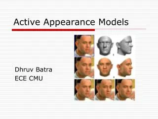
Active Appearance Model (AAM) • Erweiterung der ASM: • statistisches Helligkeitsmodel von • kompletten volumetrischen Patches um die landmarks • Form-Modell (PCA) • Ausgangsbild wird mittels Image Warping in Form gebracht • Active: Automatische Anpassung eines unbekannten Bildes mit Hilfe der gelernten Transformationen innerhalb der Limits
PDMs, ASM und AAMs • …..haben sich sehr durch ihre Robustheit bewährt • Es gibt aber natürlich auch interessante Alternativen: Statistical deformation Models, M-reps, wahrscheinlichkeitstheoretische Atlanten…
Erweiterung auf 3D und höhere Dimensionen • Absolut notwendig da moderne (medizinische) Geräte Daten in 3D und mehr bereits liefern • Schwierigkeit: Riesige Datenmengen • richtige Point Correspondence • konsistentes setzenvon Landmarks
3D Point Distribution Models (1/4) • Konturen im Training Set • einzeichnen und labeln • (flood-filling) • Anpassen der gelabelten • Formen durch eine globale • Transformation ( Translation, • Rotation und Skalierung 9 Freiheitsgrade) an ein Reference Sample (RS) aus dem Training Set.
3D Point Distribution Models (2/4) • Konstruktion eines Atlas durch Mittelung der Distanztransformation der angepassten Formen • Wiederholung bis Atlas stabil • Reference Coordinate System (RCS) • Formen werden mit Hilfe von non-rigid-registration in RCS aufgenommen • (Lokale Transformation: Free Form Deformations basierned auf B-Splines )
3D Point Distribution Models (3/4) • Das Mittel der erhaltenen lokalen Transformationen wird auf das RCS angewandt Natural Coordinate System (NCS) • Setzen von Landmarks am • Atlas (marching cubes • Algorithmus: Oberflächen- • triangulierung) • Landmark Propagation: Landmarks werden durch inverse Transformation für jede Form automatisch berechnet
3D Point Distribution Models (4/4) • PCA kann • durchgeführt • werden
3D Active Shape Models • Schlüsselkriterien: • Unabhängigkeit von der Orientierung der Bildschichten und der Art und Weise der Bilderzeugung (MR, CT) • Anwendbarkeit auf nur wenig gesampelte Daten mit beliebiger Orientierung • 2D Bilddaten zum updaten des Models • Erzeugung der Update-Punkte basierend auf RELATIVEN Farbdifferenzen
Model Matching Extract contours from mesh Align 2D-in-plane displacement vectors to 3D vertex normals Sample contours Align model mesh to displace points cloud Generate new candidate position for sample points Deform model to minimize the shape difference with the points cloud Propagate point displacements to mesh vertices Convergence? NO YES Finished
Fuzzy Inference System • Bestimmung des 2D point-displacement vectors durch Pixelklassifikation • Einteilung durch relative Farbdifferenz in • Blut- • Muskel- • oder Luft-Pixel
2D + time Active Appearance Models • Problem: MR nicht zeitkontinuierlich • Erweiterung von 2D + time modeling: • Zeitdimension in Model codiert • „landmark time frames“ • nearest neighbour interpolation • => shape und intensity vectors werden verbunden • => 2D AAM
3D AAM: Modeling Volume Appearance • intensity model • sample volumes => average shape (warping) • voxel-wise correspondence • voxel intensity: shape-free vector • Warping • Mapping-Funktion • piecewise affine warping • thin-plate spline warping
3D AAM: Modeling Volume Appearance • 3D: piecewise affine warping • Tetraeder (x1, x2, x3, x4) • Punkte im Tetraeder: x = αx1 + βx2 + γx3 + δx4 • 3D Delauny Triangulierung • baryzentrische Koordinaten
3D AAM: Modeling Volume Appearance • PDM • xi…. 3D landmark für sample i • 3D PDM • shape sample: lineare Kombination von Eigenvektoren • Warping • Ziel: shape-free intensity vectors • Normalisieren • shape-free intensity vectors auf Durchschnitts-Intensität normalisieren • Average intensity: 0; average variance: 1
3D AAM: Modeling Volume Appearance • PCA durchführen • Lineare Kombination • intensity sample => lineare Kombination von Eigenvektoren • Konkatenation • shape vectors + gray-level intensity vectors • PCA durchführen
3D Active Appearance Models: Matching • appearance model => image data • root-mean-square intensity difference minimieren • Modifizierung der affinene Transformation, der Intensity-Parameter und der Appearance-Koeffizienten • gradient descent method
Multi-view Active Appearance Models • 3D und 2D time AAMs • single image set at a time • cardiac MR • mehrere Blickwinkel • MVAAM • Zusammenhang und Korrelation der verschiedenen image sets • Information aus allen views
Multi-view Active Appearance Models • align training shapes • shape vectors kombinieren • PCA an Kovarianz-Matrix durchführen • gleich bei intensity model • cardiac MR views, linksventrikuläre Arteriendarstellung
3D + time Active Appearance Models • Erweiterung des 3D AAM frameworks • Zeitelement im Model • Objekte => time correspondence shape • texture vectors => single shape and texture vector
Referenzen • Handbook of Mathematical Models in Computer Vision • Ergänzende Papers: • T. Cootes, G. Edwards, and C. Taylor. Active appearance models. IEEE Trans. Pattern Anal. And Machine Intelligence, 23:681-685, 2001 • T. Cootes, G. Edwards, and C. Taylor. Active appearance models. IEEE Trans. Pattern Anal. And Machine Intelligence, 23:681-685, 2001 • A. Frangi, D. Rueckert, J. Schnabel, and W. Niessen. Automatic construction of multiple-object three-dimesional statistical shape models: application to cardiac modelling. IEEE Transactions on Medical Imaging, 21(9):1151-66,2002 • H. van Assen, M. Danilouchkine, F. Behloul, H. Lamb, R. van der Geest, J. Reiber, and B. Lelieveldt. Cardiac LV segmentation using a 3D active shape model driven by fuzzy inference. In Medical Image Computing & Computer Assisted Interventions – MICCAI, volume 2878 of Lecture Notes in Computer Science, pages 535-540. Springer Verlag, Berlin 2003 • S. Mitchell, J. Bosch, B. Lelieveldt, R. van der Geest, J. Reiber, and M. Sonka. 3-D active appearance models: segmentation of cardiac MR and ultrasound images. IEEE Transactions on Medical Imaging. 21(9=:1167-78, September 2002