Point Distribution Models Active Appearance Models
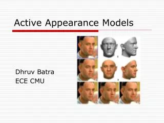
Point Distribution Models Active Appearance Models. Compilation based on: Dhruv Batra ECE CMU Tim Cootes Machester. Essence of the Idea (cont.). Explain a new example in terms of the model parameters. So what’s a model. Model. “texture”. “Shape”. Active Shape Models.

Point Distribution Models Active Appearance Models
E N D
Presentation Transcript
Point Distribution Models Active Appearance Models Compilation based on: Dhruv Batra ECE CMU Tim Cootes Machester
Essence of the Idea (cont.) • Explain a new example in terms of the model parameters
So what’s a model Model “texture” “Shape”
Active Shape Models training set
Texture Models warp to mean shape
Intensity Normalisation • Allow for global lighting variations • Common linear approach • Shift and scale so that • Mean of elements is zero • Variance of elements is 1 • Alternative non-linear approach • Histogram equalization • Transforms so similar numbers of each grey-scale value
Shape: Review of Construction Mark face region on training set Sample region Normalise The Fun Step Statistical Analysis
Multivariate Statistical Analysis • Need to model the distribution of normalised vectors • Generate plausible new examples • Test if new region similar to training set • Classify region
Fitting a gaussian • Mean and covariance matrix of data define a gaussian model
Principal Component Analysis • Compute eigenvectors of covariance, S • Eigenvectors : main directions • Eigenvalue : variance along eigenvector
Eigenvector Decomposition • If A is a square matrix then an eigenvector of A is a vector, p, such that • Usually p is scaled to have unit length,|p|=1
Eigenvector Decomposition • If K is an n x n covariance matrix, there exist n linearly independent eigenvectors, and all the corresponding eigenvalues are non-negative. • We can decompose K as
Eigenvector Decomposition • Recall that a normal pdf has • The inverse of the covariance matrix is
Fun with Eigenvectors • The normal distribution has form
Fun with Eigenvectors • Consider the transformation
Fun with Eigenvectors • The exponent of the distribution becomes
Normal distribution • Thus by applying the transformation • The normal distribution is simplified to
Dimensionality Reduction • Co-ords often correllated • Nearby points move together
Dimensionality Reduction • Data lies in subspace of reduced dim. • However, for some t,
Approximation • Each element of the data can be written
Useful Trick • If x of high dimension, S huge • If No. samples, N<dim(x) use
Building Eigen-Models • Given examples • Compute mean and eigenvectors of covar. • Model is then • P – First t eigenvectors of covar. matrix • b – Shape model parameters
Eigen-Face models • Model of variation in a region
Applications: Locating objects • Scan window over target region • At each position: • Sample, normalise, evaluate p(g) • Select position with largest p(g)
Multi-Resolution Search • Train models at each level of pyramid • Gaussian pyramid with step size 2 • Use same points but different local models • Start search at coarse resolution • Refine at finer resolution
Application: Object Detection • Scan image to find points with largest p(g) • If p(g)>pmin then object is present • Strictly should use a background model: • This only works if the PDFs are good approximations – often not the case
Back (sadly) to Texture Models raster scan Normalizations
PCA Galore Reduce Dimensions of shape vector Reduce Dimension of “texture” vector They are still correlated; repeat..
Object/Image to Parameters modeling ~80
Playing with the Parameters First two modes of shape variation First two modes of gray-level variation First four modes of appearance variation
Active Appearance Model Search • Given: Full training model set, new image to be interpreted, “reasonable” starting approximation • Goal: Find model with least approximation error • High Dimensional Search: Curse of the dimensions strikes again
Active Appearance Model Search • Trick: Each optimization is a similar problem, can be learnt • Assumption: Linearity • Perturb model parameters with known amount • Generate perturbed image and sample error • Learn multivariate regression for many such perterbuations
Active Appearance Model Search • Algorithm: • current estimate of model parameters: • normalized image sample at current estimate
Active Appearance Model Search • Slightly different modeling: • Error term: • Taylor expansion (with linear assumption) • Min (RMS sense) error: • Systematically perturb and estimate by numerical differentiation
Sub-cortical Structures Initial Position Converged
Random Aside • Shape Vector provides alignment = 43 Alexei (Alyosha) Efros, 15-463 (15-862): Computational Photography, http://graphics.cs.cmu.edu/courses/15-463/2005_fall/www/Lectures/faces.ppt
Random Aside • Alignment is the key 1. Warp to mean shape 2. Average pixels Alexei (Alyosha) Efros, 15-463 (15-862): Computational Photography, http://graphics.cs.cmu.edu/courses/15-463/2005_fall/www/Lectures/faces.ppt
Random Aside • Enhancing Gender more same original androgynous more opposite D. Rowland, D. Perrett. “Manipulating Facial Appearance through Shape and Color”, IEEE Computer Graphics and Applications, Vol. 15, No. 5: September 1995, pp. 70-76
Random Aside (can’t escape structure!) Antonio Torralba & Aude Oliva (2002) Averages: Hundreds of images containing a person are averaged to reveal regularities in the intensity patterns across all the images. Alexei (Alyosha) Efros, 15-463 (15-862): Computational Photography, http://graphics.cs.cmu.edu/courses/15-463/2005_fall/www/Lectures/faces.ppt
Random Aside (can’t escape structure!) “100 Special Moments” by Jason Salavon Jason Salavon, http://salavon.com/PlayboyDecades/PlayboyDecades.shtml
Random Aside (can’t escape structure!) “Every Playboy Centerfold, The Decades (normalized)” by Jason Salavon 1960s 1970s 1980s Jason Salavon, http://salavon.com/PlayboyDecades/PlayboyDecades.shtml