Active Appearance Models

1. Active Appearance Models AG KI, Journal Club 03 Nov 2008

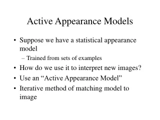
4. The Idea • Objects are modelledin shape and grey-level appearance (training necessary) • New model instances are synthesized and matched onto the new image • Model parameters are altered according to the quality of the fit

5. The Idea • Generate new model x x = μ + P*b from mean model μ and some (b) linear combination of principal components P • Fit Ix to image region Ii, by altering b according to (Ix – Ii ) = ΔI offline online

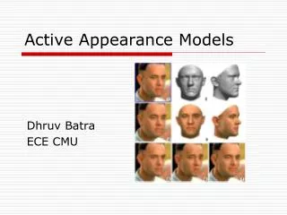
6. creating the model: step by step • annotate landmark points • align the shapes • PCA (find modes of shape variation) • make data shape-free • normalize grey values • PCA (find modes of grey value variation) • PCA (on the combined model) Example: 122 landmarks for the face image

7. What the … PCA? BASICS • Principal Component Analysis (aka: Karhunen-Loeve Transform)

8. PCA, cont. BASICS • used for decorrelation, dimension reduction, generalization • Data is assumed to be: • Linear • Gaussian (unimodal) • Principal components: eigenvectors of the Covariance matrix

9. AAMexplorer

10. Fitting the model onto the image /* reminder */ • x = μ + P*b • simplest approach: Δb = A*ΔI • „learn“ A: • perturbate known model b‘ = b + Δb and store the change of image ΔI • Find A by multi-variate linear regression • (note:) A connects grey-value appearance with all model params

11. Optimization vs. Learning Small perturbations optimum optimum Initial position

12. Extras • Iterative Approach: • b1 = b0 + kΔb with k \in {0.25, …, 2.0} • evaluate error and accept new estimate b1, if better fit, otherwise change k • Multi-resolution: use pyramids to extendthe prediction to greater ranges

13. AAMs: Properties • good results if initial guess within 20 pixels and 10% scale • depends on training image background appearance, too