Extrapolation Technique Summarized
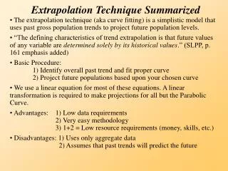
Extrapolation Technique Summarized. The extrapolation technique (aka curve fitting) is a simplistic model that uses past gross population trends to project future population levels.

Extrapolation Technique Summarized
E N D
Presentation Transcript
Extrapolation Technique Summarized • The extrapolation technique (aka curve fitting) is a simplistic model that uses past gross population trends to project future population levels. • “The defining characteristics of trend extrapolation is that future values of any variable are determined solely by its historical values.” (SLPP, p. 161 emphasis added) • Basic Procedure: 1) Identify overall past trend and fit proper curve 2) Project future populations based upon your chosen curve • We use a linear equation for most of these equations. A linear transformation is required to make projections for all but the Parabolic Curve. • Advantages: 1) Low data requirements 2) Very easy methodology 3) 1+2 = Low resource requirements (money, skills, etc.) • Disadvantages: 1) Uses only aggregate data 2) Assumes that past trends will predict the future
The Curves to Be Fit • Linear Curve: Plots a straight line based on the formula:Y = a + bX • Geometric Curve: Plots a curve based upon a rate of compounding growth over discrete intervals via the formula: Y = aebX • Parabolic (Polynomial) Curve: A curve with “one bend” and a constantly changing slope. Formula: Y = a + bX + cX2 • Modified Exponential Curve*: An asymptotic growth curve that recognizes that a region will reach an upper limit of growth. It takes the form: Y = c + abX • Gompertz Curve*: Describes a growth pattern that is quite slow, increases for a time, and then tapers off as the population approaches a growth limit. Form: Y = c(a) exp (bX) • Logistic Curve*: Similar to the Gompertz Curve, this is useful for describing phenomena that grow slowly at first, increase rapidly, and then slow with approach to a growth limit.Y = (c + abX)-1* = Asymptotic Curves
The Linear Curve (Y = a + bX) • Fits a straight line to population data. The growth rate is assumed to be constant, with non-compounding incremental growth. Calculated exactly the same as using linear regression (least-squares criterion). • Advantages: --Simplest curve --Most widely used --Useful for slow or non-growth areas • Disadvantages: --Rarely appropriate to demographic data • Example: • Y = 55,000 + 6,000(X) • In plain language, this equation tells us that for each year that passes, we can project an additional 6,000 people will be added to the population. So, in 10 years we would project 60,000 more people using this equation (6,000 * 10). • Evaluation: Generally used as a staring point for curve fitting.
The Geometric Curve (Y = aebX) • In this curve, a growth rate is assumed to be compounded at set intervals using a constant growth rate. To transform this equation into a linear equation, we use logarithms. • Advantages: --Assumes a constant rate of growth --Still simple to use • Disadvantage: --Does not take into account a growth limit • Example: • Y = 55,000 * (1.00 + 0.06)X • In plain language, this equation tells us that we have a 6% growth rate. After one year we project a population of 58,300. After 10 years we would project a population of 98,497. • Evaluation: Pretty good for short term fast-growing areas. However, over the long-run, this curve usually generates unrealistically high numbers.
The Parabolic Curve (Y = a + bX + cX2) • Generally has a constantly changing slope and one bend. Very similar to the Linear Curve except for the additional parameter (c). Growing very quickly when c > 0, declining quickly when c < 0. • Advantage: --Models fast growing areas • Disadvantages: --Poor for long range projections (familiar refrain?) --No Growth Limit --More complex • Example: • Y = 43.46 + 8.78(X) + 0.581(X2) • When X=0, Y =43.46. When X = 6, Y = 117.1 • Evaluation: Exactly the same as the Geometric Curve; good for fast growing areas, but poor over the long run.
Modified Exponential Curve (Y = c + abX ) • The first of the Asymptotic Curves. Takes into account an upper or lower limit when computing projected values. The asymptote can be derived from local analysis or supplied by the model itself. • Advantage: --Growth limit is introduced --“Best fitting” growth limit • Disadvantage: --Much more complex calculations --Misleading “Growth limit” (high and low) • Example: • Yc = 114 - 64(0.75)X • The growth limit is 114. The curve takes into account the number of time periods and as X gets larger the closer you get to the Growth limit. When X = 0, Y = 50; when X = 2, Y = 78, etc. • Evaluation: This curve largely depends upon the growth limit. If the limit is reasonable, then the curve can be a good one. Also, the ability to calculate the growth limit within the model is very useful.
The Gompertz Curve (Y = c(a) exp (bX)) • Describes a growth pattern that is initially quite slow, increases for a period and then tapers off. Like the Mod Exp curve, the upper limit can be assumed or derived by the model. • Advantage: --Reflects very common growth patterns • Disadvantages: --Getting even more complex --Misleading growth limit (limit can be high or low) • Example: • log Yc = 2.699 - 1.056(0.9221)X • The equation itself is tough to understand. When X = 0, Log Y = 1.64, so Y = 44.0 (via antilog calculation). Note: Antilog of 2.699 is 500 (the growth limit) • Evaluation: A very useful curve that can be fitted to all kinds of growth patterns. However, as with the previous curve, using an assumed growth limit can be problematic unless it is reasonable and makes sense for the case at hand.
The Logistic Curve (Y = (c + abX)-1 ) • VERY similar to the Mod Exp and the Gompertz curves, except that we are taking the reciprocals of the observed values. A very popular curve. • Advantages: --Has proven to be a good projection tool --Considered a bit more stable than the Gompertz curve • Disadvantages: --Complex! --Hard to interpret the formula • Example: • Yc-1 = 0.0020 + 0.217(0.8015)X • Another difficult to interpret equation. When X = 0, Y = 42.1. When X = 6, Y = 128.9. Note: Reciprocal of .002 is 500 (GL) • Evaluation: Considered to be the “best” of the extrapolation curves. It reflects a well-known growth pattern. It is more stable than the Gompertz curve and it does not have a misleading growth limit.
The Curve Fitting Procedure • 1) Plot the data in a chart • 2) Eyeball the data: Identify and eliminate “erroneous data”; Identify past population trends; Eliminate curves that don’t fit the data • 3) Process the data using the chosen curves, Plot your results in charts • 4) Use quantitative procedures to identify best-fitting curves • 5) Make your choice of forecast based upon a combination of quantitative and qualitative evaluations of the various projections • Many issues affect how the fit of the various curves: • --Choice of the Base Period, including the Base Year • --Calibration of projections • --Use of Growth Limits
Understanding Extrapolation • One basic principle when using the the extrapolation technique effectively is:The choice of the Base Period can have a significant impact upon the projection generated. • In the Manatee County example, if we use a varying Base Period and the Lin Reg method, we get the following results:
Improving Extrapolation Projections through Calibration • The Linear Curve also helps to illustrate one improvement to the extrapolation technique: • Oftentimes analysts “calibrate” their model to fit the projection to the observed data. • Calibration is very simply an adjustment that makes the projected population consistent with the launch year population. • Calibration is calculated by subtracting the estimated population from the observed population in the Launch Year (Observed – Estimated). • In our Manatee County example, the adjustment for BY1950 is: • Observed Pop 2000: 264,002 Estimated Pop 2000: 253,625 Calibration: +10,377 • This figure is then added to all subsequent projections using this mixture of curve type (Lin Reg) and base period (1950-2000) • Calibration is typically used with the Lin Regression technique, but can be used in others as well.
Improving Extrapolation Projections through Upper Limits • The three asymptotic curves (Mod Exp, Gompertz, Logistic) have two derivations that offer an opportunity to “fine tune” our projections : • 1) Under one approach the model itself calculates a limit to population growth. • 2) Alternatively the analyst can set an “upper limit” for the population. • This upper limit can be generated by a carrying capacity analysis (as in Monroe County (the Keys)) or from some other study that generates an upper population bound. • The concept of growth limits has been found to be very useful in projections as populations cannot grow infinitely… there is some limit to their growth. • In incorporating this concept into the extrapolation technique there is evidence that better projections are generated.
Manatee County Example BP 1950-2000 Limit Calculated by Model Upper Limit Assumed To be 1.2 Million People