Download
1 / 43
430 likes | 525 Views
Learn about identifying outliers and influential points in regression analysis, their impact on models, and methods to handle them effectively.

E N D
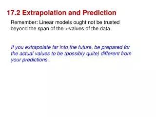
17.2 Extrapolation and Prediction Remember: Linear models ought not be trusted beyond the span of the x-values of the data. If you extrapolate far into the future, be prepared for the actual values to be (possibly quite) different from your predictions.
17.3 Unusual and Extraordinary Observations Outliers, Leverage, and Influence In regression, an outlier can stand out in two ways. It can have… 1) a large residual:
17.3 Unusual and Extraordinary Observations Outliers, Leverage, and Influence In regression, an outlier can stand out in two ways. It can have… 2) a large distance from : “High-leverage point” A high leverage point is influential if omitting it gives a regression model with a very different slope.
17.3 Unusual and Extraordinary Observations Outliers, Leverage, and Influence Tell whether the point is a high-leverage point, if it has a large residual, and if it is influential.
17.3 Unusual and Extraordinary Observations Outliers, Leverage, and Influence Tell whether the point is a high-leverage point, if it has a large residual, and if it is influential. • Not high-leverage • Large residual • Not very influential
17.3 Unusual and Extraordinary Observations Outliers, Leverage, and Influence Tell whether the point is a high-leverage point, if it has a large residual, and if it is influential.
17.3 Unusual and Extraordinary Observations Outliers, Leverage, and Influence Tell whether the point is a high-leverage point, if it has a large residual, and if it is influential. • High-leverage • Small residual • Not very influential
17.3 Unusual and Extraordinary Observations Outliers, Leverage, and Influence Tell whether the point is a high-leverage point, if it has a large residual, and if it is influential.
17.3 Unusual and Extraordinary Observations Outliers, Leverage, and Influence Tell whether the point is a high-leverage point, if it has a large residual, and if it is influential. • High-leverage • Medium residual • Very influential (omitting the red point will change the slope dramatically!)
17.3 Unusual and Extraordinary Observations • Outliers, Leverage, and Influence • What should you do with a high-leverage point? • Sometimes, these points are important. They can indicate that the underlying relationship is in fact nonlinear. • Other times, they simply do not belong with the rest of the data and ought to be omitted. • When in doubt, create and report two models: one with the outlier and one without.
17.3 Unusual and Extraordinary Observations Outliers, Leverage, and Influence WARNING: Influential points do not necessarily have high residuals and therefore can hide in residual plots. So, use scatterplots rather than residual plots to identify high-leverage outliers. (Residual plots work well of course for identifying high-residual outliers.)
17.3 Unusual and Extraordinary Observations Example: Hard Drive Prices Prices for external hard drives are linearly associated with the Capacity (in GB). The least squares regression line without a 200 GB drive that sold for $299.00 was found to be . The regression equation with the original data is How are the two equations different? Does the new point have a large residual? Explain.
17.3 Unusual and Extraordinary Observations Example: (continued) Hard Drive Prices Prices for external hard drives are linearly associated with the Capacity (in GB). The least squares regression line without a 200 GB drive that sold for $299.00 was found to be . The regression equation with the original data is . How are the two equations different? The intercepts are different, but the slopes are similar. Does the new point have a large residual? Explain. Yes. The hard drive’s price doesn’t fit the pattern since it pulled the line up but didn’t decrease the slope very much.
17.4 Working with Summary Values Scatterplots of summarized (averaged) data tend to show less variability than the un-summarized data. Wind speeds at two locations, collected at 6AM, noon, 6PM, and midnight. Raw data: Daily-averaged data: Monthly-averaged data: R2 = 0.942 R2 = 0.736 R2 = 0.844
17.4 Working with Summary Values WARNING: Be suspicious of conclusions based on regressions of summary data. Regressions based on summary data may look better than they really are! In particular, the strength of the correlation will be misleading.
17.5 Autocorrelation Time-series data are sometimes autocorrelated, meaning points near each other in time will be related. First-order autocorrelation: Adjacent measurements are related Second-order autocorrelation: Every other measurement is related etc… Autocorrelation violates the independence condition. Regression analysis of autocorrelated data can produce misleading results.
17.5 Autocorrelation Autocorrelation can sometimes be detected by plotting residuals versus time. Don’t rely on plots to detect autocorrelation. Rather, use the Durbin-Watson statistic.
17.5 Autocorrelation Durbin-Watson Statistic – estimates the autocorrelation by summing squares of consecutive differences and comparing the sum with its expected value under the null hypothesis of no autocorrelation. The value of D will always be between 0 and 4, inclusive. D = 0 perfect positive autocorrelation (et = et–1 for all points) D = 2 no autocorrelation D = 4 perfect negative autocorrelation (et = –et–1 for all points)
17.5 Autocorrelation Whether the calculated Durbin-Watson statistic D indicates significant autocorrelation depends on the sample size, n, and the number of predictors in the regression model, k. Table W of Appendix C provides critical values for the Durbin-Watson statistic (dL and dU) based on n and k.
17.5 Autocorrelation Testing for positive first-order autocorrelation: If D < dL, then there is evidence of positive autocorrelation If dL < D < dU, then test is inconclusive If D > dU, then there is no evidence of positive autocorrelation Testing for negative first-order autocorrelation: If D > 4 – dL, then there is evidence of negative autocorrelation If 4 – dL < D < 4 – dU, then test is inconclusive If D < 4 – dU, then there is no evidence of negative autocorrelation
17.5 Autocorrelation • Dealing with autocorrelation: • Time series methods (Chapter 20) attempt to deal with the problem by modeling the errors. • Or, look for a predictor variable (Chapter 19) that removes the dependence in the residuals. • A simple solution: sample from the time series so that the values are more distant in time and likely minimize first-order autocorrelation (sampling may do nothing to minimize higher-order autocorrelation, though).
17.5 Autocorrelation Example: Monthly Orders A company fits a regression to predict monthly Orders over a period of 48 months. The Durbin-Watson statistic of the residuals is 0.875. At α = 0.01, what are the values of dL and dU? Is there evidence of positive autocorrelation? Is there evidence of negative autocorrelation?
17.5 Autocorrelation Example: Monthly Orders A company fits a regression to predict monthly Orders over a period of 48 months. The Durbin-Watson statistic of the residuals is 0.875. At α = 0.01, what are the values of dL and dU? Using n = 50 from the table, dL = 1.32 and dU = 1.40. Is there evidence of positive autocorrelation? Yes. D < 1.32. Is there evidence of negative autocorrelation? No. D < 4 – 1.40.
17.6 Transforming (Re-expressing) Data Linearity Some data show departures from linearity. Example: Auto Weight vs. Fuel Efficiency Linearity condition is not satisfied.
17.6 Transforming (Re-expressing) Data y Linearity In cases involving upward bends of negatively-correlated data, try analyzing –1/y (negative reciprocal of y) vs. x instead. Linearity condition now appears satisfied.
17.6 Transforming (Re-expressing) Data The auto weight vs. fuel economy example illustrates the principle of transforming data. There is nothing sacred about the way x-values or y-values are measured. From the standpoint of measurement, all of the following may be equally-reasonable: x vs. y x vs. –1/y x2 vs. y x vs. log(y) One or more of these transformations may be useful for making data more linear, more normal, etc.
17.6 Transforming (Re-expressing) Data Goals of Re-expression Goal 1 Make the distribution of a variable more symmetric.
17.6 Transforming (Re-expressing) Data Goals of Re-expression Goal 2 Make the spread of several groups more alike. We’ll see methods later in the book that can be applied only to groups with a common standard deviation.
17.6 Transforming (Re-expressing) Data Goals of Re-expression Goal 3 Make the form of a scatterplot more nearly linear.
17.6 Transforming (Re-expressing) Data Goals of Re-expression Goal 4 Make the scatter in a scatterplot or residual plot spread out evenly rather than following a fan shape.
17.7 The Ladder of Powers Ladder of Powers – a collection of frequently-useful re-expressions.
17.7 The Ladder of Powers Ladder of Powers – a collection of frequently-useful re-expressions.
17.7 The Ladder of Powers Ladder of Powers – a collection of frequently-useful re-expressions.
17.7 The Ladder of Powers Example : Foreign Prices You want to model the relationship between prices for various items in Paris and Hong Kong. The scatterplot of Hong Kong prices vs. Paris prices shows a generally straight pattern with a small amount of scatter. What re-expression (if any) of the Hong Kong prices might you start with?
17.7 The Ladder of Powers Example : Foreign Prices You want to model the relationship between prices for various items in Paris and Hong Kong. The scatterplot of Hong Kong prices vs. Paris prices shows a generally straight pattern with a small amount of scatter. What re-expression (if any) of the Hong Kong prices might you start with? No re-expression is needed to strengthen the linearity assumption. More information is needed to decide whether re-expression might strengthen the normality assumption or the equal-variance assumption.
17.7 The Ladder of Powers Example : Population Growth You want to model the population growth of the United States over the past 200 years with a percentage growth that’s nearly constant. The scatterplot shows a strongly upwardly curves pattern. What re-expression (if any) of the Hong Kong prices might you start with?
17.7 The Ladder of Powers Example : Population Growth You want to model the population growth of the United States over the past 200 years with a percentage growth that’s nearly constant. The scatterplot shows a strongly upwardly curves pattern. What re-expression (if any) of the Hong Kong prices might you start with? Try a “Power 0” (logarithmic) re-expression of the population values. This should strengthen the linearity assumption.
Make sure the relationship is straight enough to fit a regression model. • Be on guard for data that is a composite of values from different groups. If you find data subsets that behave differently, consider fitting a different model to each group. • Beware of extrapolating. • Beware of extrapolating far into the future.
Look for unusual points. • Beware of high-leverage points, especially those that are influential. • Consider setting aside outliers and re-running the regression. • Treat unusual points honestly. You must not eliminate points simply to “get a good fit”.
Be alert for autocorrelation. A Durbin-Watson test can be useful for revealing first-order autocorrelation. • Watch out when dealing with data that are summaries. These tend to inflate the impression of the strength of the correlation. • Re-express your data when necessary.
What Have We Learned? Be skeptical of regression models. Always plot and examine the residuals for unexpected behavior. Be alert to a variety of possible violations of the standard regression assumptions and know what to do when you find them. Be alert for subgroups in the data. • Often these will turn out to be separate groups that should not be analyzed together in a single analysis. • Often identifying subgroups can help us understand what is going on in the data.
What Have We Learned? Be especially cautious about extrapolating beyond the data. Look out for unusual and extraordinary observations. • Cases that are extreme in x have high leverage and can affect a regression model strongly. • Cases that are extreme in y have large residuals. • Cases that have both high leverage and large residuals are influential. Setting them aside will change the regression model, so you should consider whether their influence on the model is appropriate or desirable.
What Have We Learned? Notice when you are working with summary values. • Summaries vary less than the data they summarize, so they may give the impression of greater certainty than your model deserves. Diagnose and treat nonlinearity. • If a scatterplot of y vs. x isn’t straight, a linear regression model isn’t appropriate. • Re-expressing one or both variables can often improve the straightness of the relationship. • The powers, roots, and the logarithm provide an ordered collection of re-expressions so you can search up and down the “ladder of powers” to find an appropriate one.