Download

1 / 28
280 likes | 315 Views
Learn to differentiate one-way and two-way ANOVA, arrange data for analysis, and test hypotheses with ANOVA techniques. Understand key terms like factor, treatment, and experimental units. Explore One-Way ANOVA in a completely randomized design and its calculations.

E N D
Learning Objectives • Describe the relationship between analysis of variance, the design of experiments, and the types of applications to which the experiments are applied. • Differentiate one-way and two-way ANOVA techniques. • Arrange data into a format that facilitates their analysis by the appropriate ANOVA technique. • Use the appropriate methods in testing hypothesis relative to the experimental data.
Factor level, treatment, block, interaction Experimental units Replication Within-group variation Between-group variation Completely randomized design Randomized block design Factorial experiment Sum of squares: Treatment Error Block Interaction Total Key Terms
Key Concepts • ANOVA can be used to analyze the data obtained from experimental or observational studies. • A factor is a variable that the experimenter has selected for investigation. • A treatment is a level of a factor. • Experimental unitsare the objects of interest in the experiment. [effect in experiment] • Variation between treatment groups captures the effect of the treatment. A : B : C [Between group-variance] • Variation within treatment groups represents random error not explained by the experimental treatments. A ONLY [Within group variance]
EXAMPLE: Mazlan studied the effect of three learning skills; peer group discussion, extra exercises, and additional reference books towards student’s score. Define which are factor, treatment and experimental units. Answer: Factor – Learning skill Treatment- peer group discussion, extra exercises, and additional reference books Experimental units - student’s score
Analysis of Variance: A Conceptual Overview • Assumptions for Analysis of Variance The populations from which the samples were obtained must be normally or approximately normal distributed The variance of the response variable, denoted 2, is the same for all of the populations. The observations (samples) must be independent of each other
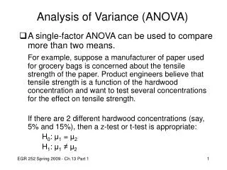
One-Way ANOVA (Completely Randomized Design) • A completely randomized design(CRD) is an experimental design in which the treatments are randomly assigned to the experimental units. • Purpose: Examines two or more levels of an independent variable to determine if their population means could be equal or not. • Effects model for CRD:
One-Way ANOVA, cont. • Hypothesis: • H0: µ1 = µ2 = ... = µt * • H1: µiµj for at least one pair (i,j) (At least one of the treatment group means differs from the rest. OR At least two of the population means are not equal) @ * where t = number of treatment groups or levels
CONCLUSION Fail to Reject H0 Reject H0 No difference in mean Difference in mean Between- group variance estimate approximately equal to the within-group variance Between- group variance estimate will be larger than within-group variance F test value = greater than 1 F test value approximately equal to 1 * Treatments are not equal * All treatments are equal
One-Way ANOVA, cont. • Format for data: Data appear in separate columns or rows, organized by treatment groups. Sample size of each group may differ. • Calculations: • Sum of squares total (SST) = sum of squared differences between each individual data value (regardless of group membership) minus the grand mean, , across all data... total variation in the data (not variance).
One-Way ANOVA, cont. • Calculations, cont.: • Sum of squares treatment (SSTR) = sum of squared differences between each group mean and the grand mean, balanced by sample size... between-groups variation (not variance). • Sum of squares error (SSE) = sum of squared differences between the individual data values and the mean for the group to which each belongs... within-group variation .
One-Way ANOVA, cont. • Calculations, cont.: • Mean square treatment (MSTR) = SSTR/(t – 1), where t is the number of treatment groups... between-groups variance. • Mean square error (MSE) = SSE/(N – t), where N is the number of elements sampled and t is the number of treatment groups... within-groups variance. • F-Ratio [ F test ] = MSTR/MSE, where numerator degrees of freedom are t – 1 and denominator degrees of freedom are N – t. - F, t-1,N-t refer table ms 30 • If F-Ratio > F or p-value < , reject H0 at the level.
One-Way ANOVA, cont. Comparing the Variance Estimates: The F Test • Sampling Distribution of MSTR/MSE Sampling Distribution of MSTR/MSE Reject H0 a Do Not Reject H0 MSTR/MSE F Critical Value
One-Way ANOVA - An Example Example 4.1: Safety researchers, interested in determining if occupancy of a vehicle might be related to the speed at which the vehicle is driven, have checked the following speed (MPH) measurements for two random samples of vehicles: Driver alone: 64 50 71 55 67 61 80 56 59 74 1+ rider(s): 44 52 54 48 69 67 54 57 58 51 62 67 a. What are the null and alternative hypothesis? H0: µ1 = µ2 where Group 1 = driver alone H1: µ1¹µ2 Group 2 = with rider(s)
One-Way ANOVA - An Example b. Use ANOVA and the 0.025 level of significance in testing the appropriate null hypothesis. SSTR = 10(63.7 – 60)2 + 12(56.917 – 60)2 = 250.983 SSE = (64 – 63.7 )2 + (50 – 63.7 )2 + ... + (74 – 63.7 )2 + (44 – 56.917) 2 + (52 – 56.917) 2 + ... + (67 – 56.917) 2 = 1487.017 SST = (64 – 60 )2 + (50 – 60 )2 + ... + (74 – 60 )2 + (44 – 60) 2 + (52 – 60) 2 + ... + (67 – 60) 2 = 1738
One-Way ANOVA - An Example Compare calculated values to those in the Excel output: The test statistic The p-value The critical bound
One-Way ANOVA - An Example • Example 4.2 : AutoShine, Inc. AutoShine, Inc. is considering marketing a long- lasting car wax. Three different waxes (Type 1, Type 2, and Type 3) have been developed. In order to test the durability of these waxes, 5 new cars were waxed with Type 1, 5 with Type 2, and 5 with Type 3. Each car was then repeatedly run through an automatic carwash until the wax coating showed signs of deterioration. The number of times each car went through the carwash before its wax deteriorated is shown on the next slide. AutoShine, Inc. must decide which wax to market. Are the three waxes equally effective?
One-Way ANOVA - An Example Factor . . . Car wax Treatments . . . Type I, Type 2, Type 3 Experimental units . . . Cars Response variable . . . Number of washes
One-Way ANOVA - An Example Testing for the Equality of k Population Means: A Completely Randomized Design Wax Type 1 Wax Type 2 Wax Type 3 Observation 1 2 3 4 5 27 30 29 28 31 33 28 31 30 30 29 28 30 32 31 Sample Mean 29.0 30.4 30.0 Sample Variance 2.5 3.3 2.5
One-Way ANOVA - An Example Testing for the Equality of k Population Means: A Completely Randomized Design 1. Hypothesis H0: 1=2=3 H1: Not all the means are equal where: 1 = mean number of washes using Type 1 wax 2 = mean number of washes using Type 2 wax 3 = mean number of washes using Type 3 wax
One-Way ANOVA - An Example Testing for the Equality of k Population Means: A Completely Randomized Design 2. Test Statistic - Mean Square Between Treatments Because the sample sizes are all equal: = (29 + 30.4 + 30)/3 = 29.8 SSTR = 5(29–29.8)2 + 5(30.4–29.8)2 + 5(30–29.8)2 = 5.2 MSTR = 5.2/(3 - 1) = 2.6 Mean Square Error SSE = 4(2.5) + 4(3.3) + 4(2.5) = 33.2 MSE = 33.2/(15 - 3) = 2.77
One-Way ANOVA - An Example Testing for the Equality of k Population Means: A Completely Randomized Design 2. ANOVA Table Source of Variation Sum of Squares Degrees of Freedom Mean Squares p-Value F 5.2 0.42 Treatments 2 2.60 0.939 Error 33.2 12 2.77 Total 38.4 14
One-Way ANOVA - An Example Testing for the Equality of k Population Means: A Completely Randomized Design 3. F value where F0.05,2,12 = 3.89 is based on an F distribution with 2 numerator degrees of freedom and 12 denominator degrees of freedom 4. Rejection Rule (Draw picture) Critical Value Approach: Do not Reject H0 if F < 3.89 p-Value Approach: Do not Reject H0 if p-value > .05
One-Way ANOVA - An Example Testing for the Equality of k Population Means: A Completely Randomized Design 5. Conclusion • F test < F alfa (3.89), do not fall in rejection region • so we do not reject H0. 2. There is insufficient evidence to conclude that the mean number of washes for the three wax types are not all the same.
EXAMPLE 2 Step 2 • 5 IMPORTANT STEP: • HYPOTHESIS TESTING • TEST STATISTIC – F TEST • F – VALUE (CRITICAL VALUE) • REJECTION REGION • CONCLUSION • SSTR - MSTR • SSE - MSE • SST = SSTR +SSE • F TEST = MSTR/MSE • BUILD ANOVA TABLE Reject H0
EXERCISETEXT BOOK PAGE 143 ( 1 & 2) • 5 IMPORTANT STEP: • HYPOTHESIS TESTING • TEST STATISTIC – F TEST • F – VALUE (CRITICAL VALUE • REJECTION REGION • CONCLUSION